ABSTRACT
This
diploma thesis studies high-speed wireless communication using the 60 GHz band.
Different aspects of such systems are reviewed, like applications, modulation
schemes and multiple access techniques. Focus is made on one application, point
to point transmission within a room. Two modulation schemes that could be used
in a future demonstrator are compared: Gaussian Minimum Shift Keying with
BT=0.5 (0.5 GMSK) and Differential Quadrature Phase Shift Keying coupled with
Orthogonal Frequency Division Multiplexing (DQPSK/OFDM). Simulations are
performed using ADS system simulation software from Hewlett-Packard.
The
emphasis is put on the system performance with respect to the characteristics
of the mm-wave MMIC circuits. In particular, we investigate the maximum bit
rate achievable, the sensitivity of the receiver regarding the received power,
to the local oscillator stability and the amplifier linearity. Different
scenarios focusing on specific parameter values are simulated to investigate limitations
of the systems.
From the
simulation results and considerations regarding hardware implementation
DQPSK/OFDM is proposed as the most suitable modulation type for 60 GHz WLAN
applications. Possible evolutions of the simulation systems are also presented.
ACKNOWLEDGEMENTS
First of all we would like to express our gratitude to our
supervisors at Ericsson Microwave Systems AB, Jonas Noréus and Arne Alping, who
have made possible this thesis project. They also advised us for the writing
and contents of the report, which with their help have been improved all along
the thesis.
We would like to thank to Arne Svensson at Chalmers University of
Technology, Dept. of Signals and Systems who accepted to be our examiner and
who has always be ready to help us on the theoretical and practical sides.
We wish to thank Herbert Zirath at Chalmers University of
Technology, Dept. of Microelectronics who provided the values for active
circuits belonging to our simulation system and made possible to implement
reliable simulation set-ups for the considered system.
Finally, we acknowledge Maxime Flament from Chalmers Signal And
Systems department who has been our supervisor during this thesis.
TABLE OF CONTENTS
ABSTRACT……………………………………………………………………2
ACKNOWLEDGEMENT…………………………………………………3
INTRODUCTION……………………………………………………………5
CHAPTER 1: OVERVIEW OF
THE 60 GHZ ISSUES…..…..8
1 Why 60 GHz for wireless COMMUNICATION ?.................... 8
2 Possible applications for a 60 GHz
communication system 10
2.1 Indoor WLAN.............................................................................. 10
2.2 In/out door, mobile/stationary........................................ 10
2.3 Point-to-point communication........................................... 11
2.4 Point-to-multipoint communication................................ 11
2.5 Choice of one application.................................................. 11
3 Worldwide institutes involved in 60 GHz
communication system RESEARCH................................................................................... 14
CHAPTER 2: TECHNICAL
ISSUES………………………………16
1 Multiple access and duplexing methods..................... 16
1.1 Multiple access methods................................................... 16
1.1.1 Frequency Division Multiple Access (FDMA)................. 16
1.1.2 Time Division Multiple Access (TDMA)............................... 17
1.1.2.1 Synchronous TDMA................................................................ 17
1.1.2.2 Statistical TDMA...................................................................... 18
1.1.3 Spread Spectrum Multiple Access (SSMA)................... 18
1.1.3.1 Code Division Multiple Access (CDMA)............................ 19
1.1.3.2 Frequency Hopped Multiple Access (FHMA)................ 19
1.2 Duplexing methods................................................................ 19
1.2.1 Time Division Duplex (TDD)..................................................... 19
1.2.2 Frequency Division Duplex (FDD)...................................... 19
1.3 Discussion................................................................................. 20
2 Modulation schemes............................................................. 21
3 Hardware parameters and circuits.............................. 24
3.1 PARAMETERS............................................................................... 24
3.2 CIRCUITS....................................................................................... 27
4 Channel model......................................................................... 28
CHAPTER 3: SIMULATION
SYSTEMS AND RESULTS..30
1 SYSTEM
OVERVIEW.................................................................... 30
1.1 Common parts between the two set-ups................... 31
1.2 GMSK
SIMULATION SETUP.......................................................... 34
1.3 DQPSK/OFDM
SIMULATION SETUP........................................... 35
2 SIMULATION
RESULTS................................................................. 36
2.1 GMSK
SYSTEM.............................................................................. 36
2.1.1 SENSITIVITY................................................................................... 37
2.1.2 PHASE NOISE INFLUENCE.......................................................... 38
2.2 DQPSK/OFDM
SYSTEM............................................................... 39
2.2.1 SENSITIVITY................................................................................... 39
2.2.2 THIRD ORDER INTERCEPT POINT (IP3).................................... 40
2.2.3 PHASE NOISE INFLUENCE.......................................................... 42
2.3 COMPARISON............................................................................... 42
CHAPTER 4: POSSIBLE EVOLUTION AND ENHANCEMENTS…………………………………...43
1 INTERLEAVING
AND CHANNEL CODING.................................... 43
2 DIVERSITY..................................................................................... 44
3 ANTENNA
CHARACTERISTICS AND MORE EFFICIENT EQUALISATION 46
CHAPTER 5: SUMMARY AND
CONCLUSION………….. 47
APPENDIX A: GMSK AND
DQPSK/OFDM MODULATIONS
1 Gaussian
Minimum Shift Keying (GMSK)...................................... 50
2 Differential
Phase Shift Keying (DQPSK) / Orthogonal Frequency Division Multiplexing (OFDM)....................................................................... 53
APPENDIX B: ADS SCHEMATICS AND IMPLEMENTATION DETAILS………………...60
1 GMSK
SYSTEM.............................................................................. 60
1.1 COMPLETE
SCHEMATIC.............................................................. 60
1.2 GMSK
MODULATOR AND UP-CONVERSION............................. 61
1.3 CHANNEL....................................................................................... 62
1.4 DOWN-CONVERSION.................................................................. 63
1.5 DEMODULATOR........................................................................... 63
1.6 EQUALISER
AND DECISION........................................................ 64
1.7 PHASE
LOCK LOOP..................................................................... 65
2 OFDM/DQPSK
SYSTEM............................................................... 66
2.1 COMPLETE
SCHEMATIC.............................................................. 66
2.2 MODULATOR................................................................................. 66
2.3 TIME
CONVERSION...................................................................... 67
2.4 DEMODULATOR........................................................................... 68
APPENDIX C: MATLAB CHANNEL GENERATION PROGRAMME……………………………………….70
REFERENCES……………………………………………………………..73
1 PUBLICATIONS.............................................................................. 73
2.1 BOOKS,
Ph.D. AND M.Sc. THESIS.............................................. 77
INTRODUCTION
Over the last years, networks have become a part of every day work
for nearly everybody. Network and computer communications are the easiest ways
to transfer documents from one computer to another and therefore from someone
to someone else who may stand in the room next to yours or in another country.
As people become more familiar with this technology, they want to transmit
increasingly large documents. From a data rate of some kbits/sec ten years ago,
the demand is presently of some Mbits/s and it continues to increase. Those bit
rates are easily implemented with wired network using coaxial cable or twisted
pairs. Nevertheless, wired network suffers two main drawbacks: the limited
bandwidth available and the setting up of the network itself in buildings,
which are not yet equipped. The use of optical fibres can solve the problem of
bandwidth for a rather high price and therefore is not a popular solution.
However, we will see later on that the Broadband Integrated Services Digital
Network (B-ISDN) standard is the basis of broadband wireless network.
Compatibility between wired and wireless network would be a great advantage for
the new coming wireless systems.
Those reasons have led companies to undertake researches about radio
or wireless networks. This type of network offers two advantages. You are not
relying on the location of your terminal, if it is placed within the range of a
base station, and a large bandwidth is available provided that you are using a
carrier frequency of some tens of GHz. For this reason, the conventional
frequency bands for mobile communication, 900 and 1800 MHz, are not suitable
because they do not allow enough spectral space. Moreover, these frequencies
are not free of use. Free frequencies and wide spectral space are available
above 25 GHz. Among these, one band is object of particular attention. The
60 GHz band, roughly between 59 and 64 GHz, has the property of being
the atmospheric oxygen absorption band. In an outdoor environment, this means
that signals are strongly attenuated, up to 15 dB/km in addition to the free
space loss. In this report, we will focus on indoor applications where
60 GHz is also severely attenuated by inner walls and human bodies. These
properties and the fact that output power will be technologically limited to
some tens of mW lead to a good frequency reuse factor.
The task of this thesis project is to set up a possible 60 GHz
wireless model and to study the influence of electronic circuits’
characteristics on the system performance. We decided to focus on a
point-to-point link for the simulations. The circuit characteristics have been
provided by Chalmers University of Technology (Gothenburg, Sweden). The
circuits have been designed using the GaAs-HEMT technology. The study has been
performed using the simulation software Advanced Design System (ADS) from
Hewlett-Packard. This software has a practical graphical interface and number
of libraries with analog and digital components already implemented.
In Chapter 1 we are discussing issues around 60 GHz, such as
possible applications and research activities worldwide.
Chapter 2 deals with more technical details like multiple access
methods, system parameters, modulation schemes, and channel model for
simulation.
Chapter 3 presents the simulation set ups as well as the comparison
results between two modulation schemes, DQPSK/OFDM and GMSK. We emphasis on the
dependence of bit error rate and therefore achievable bit rate with respect to
hardware parameters.
Chapter 4 is dedicated to the study of techniques suitable to
improve the system performances. We introduce channel coding, interleaving,
diversity and equalisation.
Finally, the main results of this project are summarised and
conclusions are drawn in Chapter 4.
CHAPTER
1: OVERVIEW OF THE 60 GHz ISSUES
· The 60 GHz band (between 59 and 64 GHz) provides an
abundance of spectral space, which is required for a high data rate (several
hundreds of Mbps). Indeed, at lower frequencies, the spectral space is already
occupied for other applications as it can be seen in figure 1.1. The
60 GHz band still being free and unlicensed, a large bandwidth, for
example of the order of 1 GHz, can easily be used.

Figure 1.1: Spectral allocation.
Figure 1.1 shows the applications commonly used depending on the
frequency band. For radio propagation, there exists a reglementation in each
country, allocating a specific frequency band for a purpose. For example, some
frequency bands have to remain free for army use, others are reserved for
maritime radionavigation. The interested reader can have a look on the frequency
allocation chart in the United States on the URL:
http://www.ntia.doc.gov/osmhome/allochrt.html
· Time dispersion of millimetre-wave channels is considerably smaller
compared with time dispersion at UHF frequencies due to a stronger attenuation.
This is not really true in an indoor environment in which there is not a large
difference between the distances of the direct path and the reflected paths as
for the outdoor case. In this case, the waves of the reflected paths in the
latter case are much more attenuated than the waves of the direct path.
· In terms of propagation, the attenuation of the 60 GHz waves
is interesting because of the strong atmospheric oxygen absorption (about
15dB/km) and high reflection (even if the latter can be neglected compared with
the former). Figure 1.2 shows the attenuation by oxygen and uncondensed water
vapour as a function of frequency. This attenuation of the 60 GHz waves implies
that a signal is often confined into a limited area. Frequency reuse can be
performed among neighbouring coverage cells, whose size might be very small
with a radius of a few kilometres outdoor. In an indoor environment, the cell
can be limited to a single room (it is then called pico-cell). Indeed, concrete
walls attenuate 60 GHz waves by 20 dB, avoiding them to interfere
with the neighbouring cells. But this means that the base station and the
remote terminal need to be in Line-of-Sight (LOS) condition, since the
attenuation caused by an obstacle between them is very strong (about 15 dB for a
human body). In a general way, everything which is larger than half the
wavelength absorbs most of the power in the given direction and reflects the
rest. At 60 GHz, the wavelength is 5 millimetres. Thus any object
larger than 2.5 mm will be considered as an obstacle.

Figure 1.2: Attenuation by oxygen and water vapour at sea level. T=20°C. Water
content = 7.5 g/m3.
Frequency reuse is possible within very short distances (a few tens
of metres), since millimetre waves do not penetrate walls significantly so that
60 GHz band channels are more suited for transmissions in confined rooms,
e.g. an office or a factory’s workroom, than in an outdoor environment.
Wireless communication systems such as WLANs are attractive because
of their layout flexibility and portability of terminals. For such short-range
indoor broadband WLAN systems, the 60 GHz frequency band offers a
significant advantage: it supplies enough bandwidth, and therefore a sufficient
data rate for transmission of various multimedia contents. For example, people
participating in a meeting in separate rooms could exchange information such as
fixed or animated pictures, data sheets and talk with high quality video
conference in almost real time through the wired external network, or even
access the main server.
We just have seen that the indoor communication system should be
used in a single room due to the strong attenuation of the waves by the walls.
The outdoor system could be used respecting two conditions:
(1)
The transmitter and the receiver
should be quite near each other because of the free space path loss and the
absorption of the waves by the atmosphere. For example, by taking an emitting power
of 20 dBm (100 mW) and a receiver sensitivity of –90 dBm, we get
110 dB for the attenuation of the channel, which corresponds to a distance
between 100 and 105 metres.
(2)
The transmitter and receiver have to
be in Line-of-Sight condition, to avoid both frequency selectivity and large
additional path loss (over 20 dB). Nevertheless, putting antennas on the
top of buildings can easily fulfil this condition.
As the link is wireless, the terminal is of course portable. During
the communication, its mobility would imply more difficulties such as a Doppler
shift and a high fade. In a room, as the speed is never important, there is a
so small Doppler shift that it does not affect the performance very much and
can be neglected. Anyway, mobility is not very useful in such an environment.
In an outdoor environment, a mobile terminal is more needed. However, the
coverage cells are very small, and the system should therefore be used over
small distances. An example of application is a wireless TV camera connected to
a temporary studio by a 60 GHz link for sports events broadcasting.
Point-to-point transmission already exists for lower frequencies.
For example, the Minilink by Ericsson works between 7 and 38 GHz and
allows wireless transmission in telecommunication networks. Operating at
60 GHz would permit the minilink system to profit of the advantages of
this frequency band as described earlier.
The difference between the point-to-point and the point-to-multipoint
communication systems is that the latter is able to transmit to several
receivers at the same time. Thus a multiple access technique is needed for the
transmission if the transmitter should handle different data transmission to
each receiver. In case of broadcasting transmission, when the same information
is sent to all the receivers, no multiple access technique is needed.
The most suitable application for a system study of a 60 GHz
wireless communication system is a point-to-multipoint Wireless Local Area
Network placed in a room, since this is the most probable application that
Ericsson will develop. In the report, we will therefore consider an indoor WLAN
for our investigations and simulations.
A fixed base station is situated in the room. The uplink
(transmission from a remote terminal to the base station) is basically a single
point-to-point transmission, as well as the downlink (from the base station to
the remote terminal). However, a network generally involves several terminals.
The up- and downlink have then to be upgraded into respectively
multipoint-to-point and point-to-multipoint transmissions. We do not focus on a
broadcasting case, hence each terminal should receive different data. The base
station should then receive (uplink) or transmit (downlink) the data to each
terminal by using a multiple access method which will be the same for both
senarios. In each case, the total bit rate of the base station has to be
divided by the number of terminals. For example, if the base station’s maximum
bit rate is 155 Mbps and the network has 5 terminals, then each terminal
will have a bit rate of 31 Mbps at its disposal.
Moreover, the network can be composed of several cells, with one
base station each. Then the communication between two base stations should be
possible, which is a point-to-point transmission. The high bit rate (at least
155 Mbits/s in our case) has not to be shared between several terminals.
However, it is very difficult to transmit such a high bit rate over a simple
channel. The common way is to divide
the channel into several sub-channels, each carrying a low bit rate. This
method requires the use of a multiple access technique. A description of the
principal such techniques as well as a discussion about which one would be the
most suitable in our case can be seen in Chapter 2 Section 1.
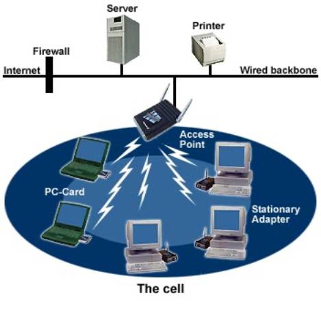
Figure 1.3: Typical senario of a WLAN.
Note that the base station is an interface either towards other
terminals or a fixed wired network as it can be seen on figure 1.3. In this
latter case, the system should be compatible with the B-ISDN standard, using
ATM technology, thus providing appropriate adaptation layer software in the
terminal. Indeed, ATM is being considered for use in fixed integrated services
local networks. Compatibility with B-ISDN enables remote stations to be easily
connected to a central server through the fixed network as mentioned in the
introduction. The WLAN should then be independent of the external operator
interface.
Integrated Services Digital Networks (ISDN)
The ISDN is intented to be a worldwide public telecommunications
network to replace existing public telecommunications networks and deliver a
wide variety of services. The ISDN is defined by the standardization of user interfaces
and is implemented as a set of digital switches and paths supporting a broad
range of traffics types and providing value-added processing services. In
practice, there are multiple networks, implemented within national boundaries,
but from the user’s point of view, there will be a single, uniformly
accessible, worldwide network.
The ISDN has been developed to transmit and process all types of
data in accordance with efficient and timely collection, processing and
dissemination of information.
The fist generation of ISDN, sometimes referred as narrowband ISDN, is based on the use of
a 64-kbps channel as the basic unit of switching and has a circuit-switching
orientation. The major technical contribution of the narrowband ISDN effort has
been Frame Relay. The second generation, referred as Broadband ISDN (B-ISDN), supports very high data rates (100s of
Mbps) and has a packet-switching orientation. The major technical contribution
of the broadband ISDN effort has been Asynchronous Transfer Mode (ATM), also
known as Cell relay.
More details about ISDN and B-ISDN can be found in [59].
Asynchronous Transfert Mode (ATM)
The ATM standard has been designed to handle high bit rate
(155.52 Mbps and 622.08 Mbps) over reliable link like optics fibre.
This means that errors are very unlikely and so very little protection has been
included in the standard. The only part of the frame protected against error is
the header. To adapt ATM to a less reliable communication medium such as
microwave, it is necessary to extend this protection. This could be done on the
physical layer by using a part of the frame space dedicated to information for
a correcting code. Reference [36] identifies Bose-Chaudhur-Hocquenghem (BCH)
code and Differential Feedback Equaliser (DFE) to be well suited for ATM cells.
Several institutes, universities and companies are undertaking
research on the 60 GHz issue. Below, we provide a non-exhaustive list of places
where investigations are taking place.
· Canada
Broadband Indoor Wireless Communications is a project sponsored by
the Canadian Institute for Telecommunication Research (CITR). A research team
is distributed among seven Canadian universities and also includes researchers
from the Communications Research Centre (CRC) and Bell-Northern Research (BNR).
· United States
The Virginia Polytechnic Institute and State University has a
project of radio link at 60 GHz.
Moreover, The Berkeley Wireless Research Center (BWRC) is designing
CMOSs for radiocommunication at 60 GHz, in collaboration with Hewlett-Packard,
Cadence, Ericsson, SGS-Thomson and Texas Instruments.
· Japan
The Communications Research Laboratory (CRL) initiated a research
project aimed at achieving a wireless LAN system in the 60 GHz band for indoor
communications operating at a transmission rate up to 160 Mbps.
· Australia
The Program for LANs and Network Services (PLANS) centred at the
CSIRO Division of Radiophysics in Australia aims to develop third-generation
wireless systems with capacities on the order of 100 Mbps in a cell.
Collaborating institutions on modulation, media-access control and networking
include:
ð CSIRO Division of Information Technology
ð Macquarie University
ð Sydney University of Technology
ð University of NSW
ð University of South Australia
· Europe
The RACE II MBS project addresses the system concepts, techniques
and technology required for the transition to Mobile Broadband System (MBS).
This project aims to develop a mobile high data rate system operating in two
subbands, 62-63 GHz and 65-66 GHz, allowing full duplex transmission. The
partners involved in this project are:
ð British Broadcasting Corporation
ð British Telecom
ð Companhia Portuguesa Radio Marconi (CPRM)
ð Deutsche Aerospace
ð Instituto Superior Tecnico
ð LEP / Philips Microwave
ð Norwegian Telecom Research
ð Technical University of Aachen
ð Thomson-CSF Semiconducteurs Spécifiques
ð VTT Technical Research Centre Finland
The RACE II project was followed by the ACTS and IST projects.
More details about the MBS project can be found at the URL:
http://www.comnets.rwth-aachen.de/project/mbs
http://www.comnets.rwth-aachen.de/project/mbs/publications/60GHz/60GHz.html
Other institutes that are making some research in the field:
ð KTH, royal institute of technology, Stockholm
http://www.s3.kth.se/radio/Research/research.html
ð PCC, Personal Computing and Communication
http://www.s3.kth.se/radio/4GW/
ð MEDIAN, Institute of mobile and satellite communication techniques,
Germany
Table 1.1: Summary of the different
systems using the 60 GHz band investigated worldwide.
|
Invented region
|
Europe (MBS)
|
Canada
|
Japan
|
Australia
|
|
Operator
|
public, private
|
private
|
private
|
private
|
|
Data rate
|
155 Mbits/s
|
155 Mbits/s
|
155 Mbits/s
|
100 Mbits/s
|
|
ATM support
|
yes
|
yes
|
|
yes
|
|
Mobility
|
up to 100 km/h
|
portable
|
portable
|
2 m/s
|
|
Applications
|
in- / outdoor
|
indoor
|
indoor
|
indoor
|
|
|
all business sectors
|
office
|
office
|
office
|
|
Frequency bands
|
62-65 GHz
|
20-65 GHz, IR
|
59-64 GHz
|
60 / 40-65 GHz
|
|
Modulation
|
16OQAM/4OQAM
|
BPSK
|
BPSK
|
|
|
Access method
|
TDMA
|
TDMA
|
TDMA
|
TDMA
|
|
Duplex method
|
FDD
|
TDD
|
|
|
|
Number of channels
|
34
|
|
|
|
|
Channel allocation
|
dynamically
|
fixed
|
|
Dynamically
|
|
Handover
|
yes
|
|
|
|
CHAPTER
2: TECHNICAL ISSUES
The multiple access is required for a point-to-multipoint
communication, i.e. between a base station and several terminals. Because the
aim of a multiple access is to provide a simultaneous transmission to every
terminal with the best reliability, many schemes have been designed during the
years. Presently, three main multiple access methods exist, FDMA, TDMA and
CDMA. A fourth method is being developed: it is based on spatial division
(SDMA) and therefore uses a sectored antenna [43]. This method is developed to
enhance the frequency reuse. Our main goal is to achieve the highest possible
data rate. Therefore, we will limit our investigation to the first three
methods because SDMA is not of very much interest in our case, given the small
size of the cells and the will to keep the system as simple as possible. More
details about multiple access and duplexing methods described in this section
could be found in [57] and [59].
First, we give an overview of the available access and duplexing
methods, with their advantages and drawbacks; then follows a discussion about
their feasibility to achieve high data rates.
FDMA is the simplest and the oldest multiple access method. Each
user receives a frequency to transmit and receive data. The main drawback of
this method, in addition to the bandwidth occupancy, is that in order to
achieve good power efficiency, the amplifiers and antennas are used at
saturation. This introduces a spreading in the frequency domain and therefore a
higher level of inter-carrier interference. To keep this level of ICI low
enough, a guard band is inserted between the uplink and the downlink. This
participates to the spectral inefficiency of the method.

Figure 2.1: Principle of (a) FDMA and
(b) TDMA, taken from [59].
For synchronous TDMA, each user has an allocated
time slot to transmit (see figure 2.1 (b)). The time slot is available but must
not necessarily be used. Due to the large bandwidth allocated to one user
during one time slot, more severe Inter-Symbol Interference (ISI) occurs. The
most known applications of TDMA are ISDN and GSM.
In synchronous TDMA, when a user is not
transmitting, its time slot is wasted. One method to increase the performance
is referred as statistical TDMA. This method is based on the fact that if one
user is not transmitting during its time slot, the slot is given to another
user. Of course, it requires more overheads to keep track of the frames, but it
increases the efficiency of TDMA. Some satellite TV operators use this method.
For simulated results of an algorithm managing statistical TDMA see [47].

Figure 2.2:
Synchronous and statistical TDMA, taken from [59].
The SSMA method has raised with the development of military mobile
communication and the third generation of mobile communication. Indeed, it is
very robust and immune to multipath interference and Doppler shift which are
the two main limiting factors of this kind of communication. However, at
60 GHz, the main problem is the multipath propagation that introduces
large delays, compared to the bit duration, in the received signal. Many users
can share the same spread spectrum bandwidth. The only limiting factor on the
number of users is the quality of transmission, which decreases with the
increase of the number of users. The main drawback of this method is that the
bandwidth required is much larger than TDMA or FDMA. Nevertheless, the
bandwidth efficiency increases with the number of users.
CDMA is the most common and a very popular scheme used in SSMA
methods. It is based on the fact that each user owns a pseudo random code word
that commands the frequency spreading. Any such code word is approximately
orthogonal to the others. This means that with a correlator receiver, i.e. RAKE
receiver, one user can hardly interfere with another user. RAKE receiver
extracts user’s signal, while other users signals are considered as white
noise. Wideband CDMA (W-CDMA) is used in the third generation of wireless
systems.
In FHMA, the frequency band is periodically changed to deal with
fading. The hopping rate can be slow if the time between two hops is longer
than one symbol time, or fast if time interval between hops is smaller than the
symbol duration.
TDD is a method by which the up-link and the
downlink share the same carrier. This leads to the fact that you need a bit
rate twice the one for Frequency Division Duplex (FDD) to achieve the same
performance, which of course is not good from ISI point of view. It also leads
to an increased equaliser complexity. One advantage of this duplexing method is
the possibility to avoid the use of a duplexer. The use of a single filter for
the whole bandwidth is also a reduction of the complexity. Moreover, antenna
diversity can be implemented in the base station. The different signals are
combined at the receiving station using diversity techniques. This is less
complex than for FDD where diversity has to be implemented at the remote
terminal.
Due to the higher bit rate, the equaliser training
sequence is longer than for FDD. In case of ATM, duplexers are needed because
the scheme states that cells must be transmitted and received at the same time
[62].
In FDD, each user has its own channel, which contains two
frequencies: one for the uplink and one for the downlink. This fact implies
that an additional guard band must be respected to avoid interference and that
the RF filtering will be handled by two filters, each having half of the total
RF bandwidth. On the other hand, by dividing the bit rate by two you reduce ISI
and so the complexity of the equaliser. Implementation of diversity is more
complex than for TDD. Here, you have to implement antenna diversity on the
terminal side [62].
From the points stated above, it is clear that if we want to achieve
high bit rate we will encounter high level of ISI. Therefore, the use of
TDMA/TDD is not well suited to a high bit rate because the one required is
twice higher than for FDD. However, in the case of Orthogonal Frequency
Division Multiplexing (OFDM) modulation, it might be possible to use this
scheme by increasing the size of the cyclic prefix. See Chapter 2 Section 2 and
Appendix A for more details about OFDM modulation.
In [48], FDM/TDMA/TDD with Gaussian Minimum Shift Keying (GMSK)
modulation is investigated and simulated in a slowly fading Rayleigh channel.
The simulations and measurements show an irreducible error floor at 5*10-3.
This system is based on the Digital European Cordless Telephone (DECT) standard
for cordless telephony. They show that the error floor is, to first order, a
function of the delay spread. However, this result is hardly extendible to our
case for at least three reasons: the carrier frequency used is 1680 MHz,
the bit rate involved is 1 Mbits/s and the channel delay profile is far
too different from ours.
In our case, we are facing two scenarios: one is the transmission
between the base station and the terminals (up- and downlink) and the other is
base station to base station communication.
For the former, the simplest as well as the most efficient would be
FDMA/FDD. Each terminal gets a pair of frequencies: one for the transmission
and one for the reception. It only needs equipment to generate one frequency
and to receive another one. The base station needs to receive the emitting
frequency of each terminal and to transmit on the receiving frequency of each
terminal.
For the latter, the bit rate required should be as high as possible
in order to handle all access demands. This requirement could be reached with
TDMA/FDD over several channels. This method has been chosen for the MBS project
[7] with 32 channels carrying up to 34 Mbits per channel. Moreover,
to be compatible with the ATM standard, the TDMA choice is a good solution
because it will only require switching the protocol and not the physical layer.
Thus, it is possible to have very high bit rate at the price of a slight
increase of the base station.
An extensive number of articles have been published on different
solutions which, could be implemented to perform a high data rate WLAN using
CDMA. Here follows a summary of the most relevant articles, also listed in
References under the title “Multiple access and duplexing methods”.
In [40], the authors propose CDMA/TDD associated with OFDM. Their
system is based on a cyclic extension of the spreading code. Computer
simulations are given for different scenarios (Doppler shift, used code,
channel).
In [44], CDMA is proposed for broadband communication. It is shown
that with a small processing gain, this system does not offer acceptable
performances. However, sectored antennas and power control are foreseen to
improve the performances. This article stress on network performance indicators
like blocking and dropping probabilities unlike the others in which BER is the
common performance measure.
Reference [41] introduces CDMA/OFDM/SFH as possible solution for
multiple access system. This is nearly an ideal solution because CDMA is well
suited for numerous users, OFDM provides a good solution to handle multipath
propagation and SFH eases the synchronisation. Apart from these ideal points,
it might be a complex system to implement. A comparison with DS-CDMA, SFH-CDMA,
MC-CDMA and OFDM-SFH is given as well as performances with channel coding over
Rayleigh fading channel.
In conclusion, if we keep in mind that a simple system is more
suited then we restrict ourselves to use TDMA or FDMA. Given the large
bandwidth available FDMA/FDD seems to be a reasonable choice. This scheme
allows transmission and reception at the same time. With 5 GHz bandwidth
and 150 Mbps for both up-link and downlink, 15 users can share the
same cell. Due to the small size of the cells, it is very unlikely that so many
users will use the whole bandwidth. That means that the bandwidth per user can
be increased.
The number of modulation schemes available is very large and every
day new schemes are proposed to cope with different situations, i.e. spectral
efficiency or robustness against a fading channel. None of them are perfect so
choosing one is always a trade-off between the main goal and the drawbacks of
the modulation scheme one has to take into account.
The design of a 60 GHz system is restricted by hardware limitation.
In our case, we focus on three parameters. The first one is power efficiency,
since the available power amplifier cannot provide more than 100 mW at
60 GHz. Moreover, it is always cheaper to build efficient non-linear
amplifiers than linear amplifiers. The second relevant parameter is the
possibility to use non-coherent detector in order to simplify the receiver
design. Finally, there is a need for a scheme that is robust against frequency
selective channel.
We could not investigate all the schemes. Therefore, we listed the most
common modulation types and figured out their main caracteristics. These
characteristics have been taken from [56], [57] and [61]. They are summarised
in the Table 2.1.
One important goal in a digital communication system is the
provision of reliable performance, exemplified by a very low probability of
error. Another important aim is the efficient utilisation of channel bandwidth.
For our project, we chose to study two bandwidth-conserving schemes for the
transmission of the binary data.
From Table 2.1, we decided to compare two
modulation schemes : DQPSK/OFDM and GMSK. The latter is widely used for
mobile communication, i.e. in the GSM and DECT standards, and fulfils all our
requirements concerning the amplification. The former has been proven robust
against channel selectivity. It is also a comparison between a multi-carrier
and a single carrier scheme. They require different processing on the receiver
side. GMSK need to be equalised since it is a single carrier scheme and so will
suffer more severe ISI. On the other hand, DQPSK/OFDM does not need to be
equalised but it is likely that an error correcting code will be needed. Deeper
details on both modulation schemes are given in Appendix A. See Chapter 4
for an introduction to error correcting codes.
A number of articles dealing with different scenarios and modulation
schemes have been published. Here is a short summary of the most interesting
ones regarding our subject.
In [25] and [27], two reduced complexity detectors of GMSK are
proposed and are shown to perform within 1 dB range of the optimum
coherent receiver for [25] and within 0.24 dB range for [27]. The
simulations are run under AWGN channel and slowly fading Rayleigh Channel.
Reference [26] shows that 0.5 GMSK has the same performance as BPSK
with perfect synchronisation. It is also shown to be more sensitive to carrier
phase error but much more robust to symbol timing error.
Reference [39] compares 0.3 GMSK with an 8-DPSK/Trellis Coded
Modulation (TCM). The latter is shown to be more spectrally efficient than
GMSK. The two systems are compared for different channels and speeds. TCM
performs better at low speed (32 km/h) with low to medium SNR and no Co-Channel
Interference (CCI) while GMSK is better for every speed up to 150 km/h in
presence of CCI. That tends to prove that GMSK is less sensible to Doppler
shift than 8-DPSK/TCM.
The influence of antenna placing and beam shape is discussed in [12]
with DQPSK/OFDM. The best results are found for an antenna standing in the
centre of the room with a sharp beam directed towards the transmitter. The
channel used is based on Saleh-Valenzuela model with parameters derived from
measurement results.
Table 2.1: Modulation Schemes characteristics
|
Modulation type
|
Pros
|
Cons
|
|
MSK
|
Constant envelope
Non-coherent detection
Non-linear amplification
|
Less spectrally efficient than QPSK and BPSK
|
|
GMSK
|
Excellent spectral efficiency
Non-coherent detection
Constant envelope
|
Receiver signal processing for high bit rate
|
|
MPSK
|
Spectrally efficient with M ¾ 4
|
Coherent detection
Linear amplification
|
|
MDPSK
|
Non-coherent detection
Better than MPSK over fading channel
|
Power efficiency lower than MPSK
|
|
MQAM
|
In AWGN channel; better than MPSK for equal M
|
Energy per symbol is not constant
Coherent detection
|
|
MFSK
|
Power efficient
Non-linear amplification possible
|
Bandwidth inefficient
|
|
OFDM (must be used together with another modulation scheme)
|
Robust against channel selectivity
|
Large average to peak power ratio -> Linear amplification
|
|
Trellis Coded Modulation (can be used together with another
modulation scheme / OFDM possible)
|
Modulation and channel coding are performed at the same time
Viterbi decoding
|
Coding and decoding more complex
|
Reference [30] investigates OFDM with higher modulation (16, 32, 64,
256-QAM and 8-PSK) schemes with a system based on IRIDIUM system, which is a
satellite network for telecommunications. TCM/OFDM gives better results than
convolutional encoded/OFDM with a lower complexity.
Reference [38] estimates and simulates 16-QAM/OFDM with
convolutional encoding over multipath channels. A Bit Error Rate equal to 10-3
is achieved with SNR equal to 19 dB.
The main task of our work was to estimate the requirements that the
electronics circuits must fit to achieve wanted performances.
The circuits used are from research laboratories at Chalmers
University of Technology. They have been designed using the GaAs-HEMT
technology. We had at our disposal data for IF and power amplifier, RF mixer,
Low Noise Amplifier (LNA) and local oscillators. Below follows a description of
the most important hardware parameters that must be considered in a
communication system, and a qualitative description of the available circuits.
Noise Figure
All electronic components generate thermal noise, and hence
contribute to the noise level seen at the detector output of a receiver. The
noise figure, denoted F, is defined by
 (2.1)
(2.1)
or by
 (2.2)
(2.2)
where Te is the device effective noise temperature and T0 the room temperature in Kelvin.
The noise power at the output of a receiver is given by
 (2.3)
(2.3)
where k is the Boltzmann’s
constant equal to 1.38*10-23 Joules/Kelvin, B is the equivalent bandwidth of the receiver and
Gsys the overall received gain.
These definitions have been taken from [57]. An example to compute Te
and F in the case of a cascaded system can be found in the same reference.
In most of the cases, the first element of the receiver’s chain
gives the highest contribution to the noise power. That is why this first
element is always a low noise amplifier. One possibility to reduce noise power
is to cool the device.
1 dB-Compression Point and
Third Order Intercept Point (IP3)
1 dB-compression point in the characteristic of an amplifier, Vout
versus Vin, where the real characteristic is 1 dB away from the
ideal one as it can be seen in Figure 2.3. It defines the linearity of the
amplifier.

Figure 2.3: Characteristic of an
amplifier.
X-axis:
input power (dBm)
Y-axis:
output power (dBm)
The IP3 level is the intercept point between the ideal linear output
and the third intermodulation product level. By rule of thumb, there are
10 dB difference between the 1 dB compression point level and the IP3
level.
Phase Noise
Phase noise describes the stability of the local oscillator around
the centre frequency. It is an important parameter because its influence on the
decoding is very high and appears at different stages. For example, the up- and
down-conversion with the mixer, if not performed at the same frequency, results
in phase error on the receiving side. The best way to avoid this error is to
use a coherent detector, where the carrier frequency used to down-convert the
signal is extracted from the signal itself. Another place where frequency
stability is important, is the sampling device reference oscillator. The
deviation of the sampling instant leads to a non-fulfilment of the Nyquist
criterion for ISI cancellation (see [56] for further details). A possible solution
to this problem is to introduce synchronisation pilot at known instant in the
transmitted data. They are used to synchronise a clock recovery device, i.e. a
Phase Lock Loop (PLL).
The unit that describes the phase noise is the decibel to carrier
(dBc). It is the ratio of the carrier power at an offset frequency from the
centre value divided by the power at the centre value.
The two spectra in figure 2.4 show the effect of phase noise on an
ideal oscillator. From a Dirac function the phase noise widens the spectrum.
The center frequency is 5 GHz and the phase noise profile is –70 dBc
at 100 kHz and –90 dBc at 10 MHz.

Figure 2.4: Spectrum of (left) an ideal
oscillator, (right) an oscillator with phase noise.
Filter Pass Bandwidth
In order to keep the noise as low as possible, the bandwidth of the
filters must match the spectrum of the signal. All the filters have the same
bandwidth but not the same frequency bandwidth. The requirement is that the
magnitude profile of the pass bandwidth must be as flat as possible. The
spectrum must be kept intact until the noise level.
Output Power
Parameter of the power amplifier on the transmitter side. However,
at very high frequencies, it is difficult to obtain high power, i.e. the
amplifier we simulate has an output power in the range from 10 to 30 mW.
The more power we have on the transmitter side, the farther we can transmit or
the easier is the demodulation process.
Amplifiers
For the amplifiers, the most relevant parameters are gain, noise
figure and output power for the power amplifier.
In our model, we use three different amplifiers: a low noise
amplifier, an intermediate frequency amplifier and a power amplifier. Their
characteristics are given in table 2.2.
Table 2.2: Amplifier characteristics
|
|
Gain (dB)
|
Noise figure (dB)
|
1 dB compression (dBm)
|
|
Low Noise Amplifier
|
17
|
5*
|
7
|
|
IF Amplifier
|
23
|
2.7
|
17
|
|
Power amplifier
|
15
|
7*
|
9
|
Oscillators
The important parameter for this device is the frequency stability
called phase noise. It quantifies the deviation of the carrier frequency around
the centre frequency. If the noise is too high it can result in an improper
demodulation at the mixer stage.
The HF modulation is performed with a 7 GHz local oscillator
multiplied by 8. The phase noise expected is –100 dBc at 100 kHz.
Mixers
Many parameters can be set, but the most important are conversion
loss and noise figure.
The typical values we got are 7 dB for the conversion loss and
7 dB for the noise figure. The conversion loss must be included in the
link budget and it is the choice of the designer to compensate it.
Most of the problems we can encounter with radio systems are coming
from the channel. That is why it is important to have a good model to validate
the system simulation. In the configuration we chose to focus on, the channel
has been proved to be slowly timed varying. Many studies have addressed
statistical or deterministic models able to predict wave propagation behaviour.
The deterministic models are strongly correlated to the environment
and to the wavelength. In example, they are taking into account furniture, size
of the room or dielectric characteristics of the building materials. Most of
these models are using ray-tracing software to model the propagation path and
loss [11,14,18,20]. At 60 GHz, waves are propagating almost like light and
so geometrical optics propagation model may be applied. These models offer very
good accuracy for a given scenario but are hardly extendable to other
situations. In Japan number of studies on material dielectric and attenuation
characteristics have been conducted [51-55].
Statistical models on the other hand are based on probability
distributions that have been shown to match measurement results. They are less
accurate than deterministic models but may be applied in many cases just by
changing a few parameters. In the UHF band where signals are more likely to
propagate through walls and on longer distance than in the EHF band, it is more
difficult to make a deterministic model since the distance involved are much
greater.
In simulation involving the UHF band, A.A.M. Saleh and R.A.
Valenzuela in [9] have proposed a model made to fit their measurements. Results
show that: (a) the indoor radio channel is quasi-static or very slowly time
varying, and (b) the statistics of the channel impulse response is independent
of transmitting and receiving antenna polarisation, if there is no LOS path
between them. The model assumes that the multipath components arrive in
clusters. The amplitude of the received components are independent Rayleigh
random variables with variance that decay exponentially with cluster delay as
well as excess delay within a cluster. The cluster and components within a
cluster form a Poisson arrival process with different rates and have exponentially
distributed interarrival times. The figure below clarifies these remarks. The
phase angles are independent uniform random variables over [0;2p]. Previous
paragraph is taken from [57].

Figure 2.5: Rays arrival time scheme,
taken from [9].
Extensions to this model have been published over the past years in
[10,12,17] for example. The most interesting is [12] because it deals with the
application of this model to 60 GHz propagation in an indoor environment. In
particular, they give parameters to apply the model at 60 GHz. It has been
proposed in [17] to model the ray phase within a cluster as a zero mean
Laplacian distribution instead of the uniform distribution.
The choice of a model depends on how much computational time that
can be spent to evaluate your channel. For example, a ray tracing software will
calculate the strength and phase of the signal every centimetre or whatever
step you choose and that will take some time to be performed. A statistical
model generates a channel in less than one second.
More
models can be found in [13,15,16,19,21].
CHAPTER
3: SIMULATION SYSTEMS AND RESULTS
The simulation set up follows the classical scheme of a
communication system depicted by Shannon in the late 1940’s. It is drawn on
Figure 3.1.

Figure 3.1: Communication system block
diagram.
Digital source: Every kind of data that
are represented in digital form. For example, it can be computer files or voice
quantized with an analog to digital converter.
Source encoder: This stage is used to
remove the redundancy in the incoming signal and then allow a larger bit rate
in the same bandwidth. A number of algorithms exist, the most common is the
Huffman algorithm but it is rarely used in its basic form due to different
lengths of output code word.
Channel encoder: This stage minimises
the effects of the noise, that is provides a reliable communication in a noisy
environment. To achieve this, controlled redundancy is added to the bit
sequence. Some more details are available in Chapter 4.
Modulator: Modulates one or more
parameters of a sinusoidal carrier with the input signal according to certain
rules. The modulated parameters can be amplitude, phase or frequency. Basic
schemes perform the modulation on only one parameter but advanced schemes can
use two parameters together (for example, 16 QAM uses phase and amplitude).
As it has been explained, we have simulated two different modulation
schemes. These two schemes do not have the same characteristics, therefore the
two simulation set-ups are slightly different.
We performed system simulations with GMSK and DQPSK/OFDM modulation
schemes.
Given that the aim of this thesis is to evaluate the influence of
some components, we used the same up/down-conversion and the same channel model
for both systems. In that way it is possible to identify the main influence and
to compare the schemes.
Figure 3.2 depicts the up-conversion. The input is an intermediate
frequency signal at 5 GHz. This one is mixed with a local oscillator at
56 GHz (7GHz*8). The resulting signal is then at 61 GHz. It is first
power amplified and then sent through a Butterworth bandpass filter.
The IF can be chosen as whatever value between 3 and 8 GHz
given that the spectrum laying from 59 GHz to 64 GHz is free of use.
The only thing to take into account is the bit rate. In critical situation,
that is when the mixer performance is poor, it is possible to perform a direct
up-conversion to 60 GHz, thus avoiding the use of a mixer.

Figure
3.2: Up-conversion.
After the transmitter, the signal goes through the channel. This one
has been generated as in Chapter 2 Section 4. Table 3.1 gives the channel’s
coefficients and Figure 3.3 shows the channel magnitude profile. The channel is
modelled as a FIR filter and followed by an attenuation factor equal to
80 dB for all the simulations except the ones investigating the sensibility
of the receiver. The program that generated the channel is given in Appendix C.
Table 3.1: Channel coefficients.
|
Delay (ns)
|
Coefficient (Complex)
|
|
0
|
1
|
|
3
|
0.1412 + i*0.1253
|
|
16
|
0.4406 + i*0.3947
|
|
18
|
-0.3605 + i*0.0412
|
|
33
|
0.0421 – i*0.0580
|
|
42
|
0.0015 – i*0.0144
|
|
44
|
0.0035 + i*0.0062
|
|
51
|
0.0026
|
|
58
|
0.0004 – i*0.0039
|
|
63
|
0.0023 + i*0.0011
|

Figure 3.3: Magnitude profile of the
channe.
X-axis: Time (ns), Y-axis: Magnitude (dB).
The receiver part is a bit more complex (Figure 3.4). The first
stage is a Butterworth bandpass filter followed by a low noise amplifier. The
filter has the same properties as the one in the transmitter. Then, the signal
is down-converted to IF. This IF signal is filtered, amplified and finally sent
to the demodulator.
 Figure 3.4: Receiver, down-conversion and
amplification.
Figure 3.4: Receiver, down-conversion and
amplification.
The 0.5 GMSK system (see Appendix A) uses a basic modulator
made of a Gaussian low pass filter driving a FM modulator. The source is
differentially encoded before being fed into the modulator.
The difference between this schematic and the general system
explained above is that the channel coding is not used. On the other hand, an
adaptive equaliser using the Least Mean Square (LMS) algorithm is part of the
detector to cope with ISI introduced by the channel.
The first part of the demodulator (Figure 3.5) is a carrier recovery
device used to track the IF carrier. With this kind of device it is possible to
cancel carrier shift due to instability in the transmitter oscillator. The same
component performs a clock recovery at half the bit rate.

Figure
3.5: Demodulator and equaliser.
The carrier recovery device used is a Phase Locked Loop (Figure
3.6). It permits to keep track of the input signal phase. So, it extracts the
carrier frequency from the input signal. The ADS PLL implementation is depicted
in Appendix B.

Figure 3.6: Block
diagram of a PLL
Once the carrier has been recovered, the IF signal is converted to
baseband and low pass filtered. Then it is fed into the complex equaliser
before a decision is done (one or zero). Some other systems perform carrier
recovery and symbol synchronisation but the PLL is the simplest one. The
interested reader will have a look in [58] Chapter 5 for example.
The gain control does not measure the signal level but keeps the
overall gain constant when some parameters involved are changed. However, it is
an important device, which is included in most radio communication equipment.
Before applying the Inverse Fast Fourier Transform (IFFT), the
signal is baseband-modulated into DQPSK: it is first mapped into a QPSK
constellation and then differentially encoded. Therefore the change of phase is
encoded: for example, one gets 11 as input bits for a phase change of 180
degrees compared with the phase of the previous symbol.
Then the IFFT is applied on the signal on 256 points and a cyclic
prefix is added to avoid intersymbol and intercarrier interference. This cyclic
prefix consists in adding some of the last coefficients (corresponding to the
time dispersion of the channel) of the OFDM sysmbol at the beginning. Numeric
OFDM symbols, each composed of 256 coefficients plus the cyclic prefix, are
then obtained. These coefficients are time-converted, before the new signal is
up-converted, in order to be transmitted through the channel. More details
about OFDM can be found in Appendix A or in [64].
The receiver part is the symmetric of the transmitter part: the
signal is down-converted from the RF to the IF and converted into numeric.
After removing the cyclic prefix, the Fourier Transform is applied to the
signal. At this stage, the signal constellation should be the same as the one
before applying the IFFT in the transmitter part, with some distortion due to
the filters and the channel. The decision on the output bits is done after the
differential decoding of the complex signal.
In order to enhance the system, a channel equaliser can be added in
the receiver part after the Fourier Transform.
Figure 3.7 shows a diagram of the transmitter part.
Bit IF Channel
Source 61 GHz
Figure 3.7: DQPSK/OFDM transmitter.
In order to ease the detection of the system weakness, the
simulations have first been run with only one parameter varying at the time. To
determine and to quantify this influence, sweep simulations of 1000 samples
each with the parameters of interest have been performed. Therefore, a BER of
10-3 is the best we can get due to simulation time. That is, a
result of 10-3 for the BER can be found lower with a longer
simulated sequence.
The first point is to see how the system behaves without phase noise
and with a received power well above the noise floor (about 40 dB). In
this basic scenario, the equaliser has 100 taps and the channel is as described
in Chapter 2 Section 4. In the equaliser, spacing the taps for more than one
sample could dramatically reduce their number. The sampling clock is assumed to
be perfectly synchronised with the signal. The chosen bit rate may seem to be
odd but it is due to the simulator where we define the symbol time rather than
the bit rate. The matching symbol time is given in the second column.
Table
3.2: BER as a function of the bit rate.
|
Bit Rate (Mbps)
|
Symbol Time (ns)
|
BER
|
|
166.66
|
6
|
10-3
|
|
250
|
4
|
10-3
|
|
666.66
|
1.5
|
10-3
|
|
1000
|
1
|
5.10-3
|
This table shows that the system has no problem to reach 1 Gbps. In
particular the two basics ATM bit rates are supported without errors.
Henceforth, the bit rate in all simulations will be 666.66 Mbps.
The sensitivity parameter shows how much attenuation the system can
cope with. There are two cases whose results are obvious. If the signal power
is well above the noise power, there is no problem to recover the signal.
Alternatively, as soon as the signal power is below the noise level, there is
no simple way to recover it from the noise. The interest is to determine where
stand the limits between these two cases. We solve this question by making a
sweep simulation through the attenuation factor.
The basic result is that the noise floor is lying around
–102 dBm. The following table shows BER as a function of the pathloss. It
is clear that the BER starts to deteriorate when the receiving power is below
–85 dBm. In this scenario, we assume perfect carrier generation and
recovery. At the output of the transmitter the signal power is 10 dBm. The
circuits have noise figure listed above.
Table 3.3: BER as
a function of the received power.
|
Received Power (dBm)
|
BER
|
|
-60
|
10-3
|
|
-80
|
10-3
|
|
-86
|
5. 10-2
|
|
-90
|
0.1
|
|
-100
|
0.3
|
Once the system sensitivity is known it is possible to prepare a
link budget.
The phase noise influence is really dependent on the characteristics
of the PLL because this one is able to track the frequency in a certain range
and with a certain speed. Once the shift is beyond this range, the system loses
its synchronisation. Of course, the action range of the PLL can be set as
wanted by the user. Therefore, it is a trade-off between spectral purity of the
generated carrier and capability to track frequency far from the reference. The
phase noise is applied at the up and down conversion with the same parameter
but not the same component. The component uses the parameter to generate a
random phase noise.
We divided the simulations into two series, one perfect oscillator
(no phase noise but no tracking of the phase) and one with the PLL (phase noise
and tracking of the noise). The phase noise profile is constituted of two
points. One is constant at 10 MHz and is equal to –100 dBc. The power
of the second is variable and is simulated from –100 dBc at 100 kHz.
Table 3.4: BER as a function of phase
noise.
|
Phase noise at 100 kHz (dBc)
|
BER with perfect oscillator
|
BER with PLL
|
|
-100
|
10-3
|
10-3
|
|
-90
|
10-3
|
10-3
|
|
-80
|
5.10-3
|
10-2
|
|
-70
|
0.1
|
5.10-2
|
|
-60
|
0.33
|
0.2
|
The PLL generates a carrier with phase noise having the following
characteristics: -40 dBc at 100 MHz, -95 dBc at 1 GHz. The
spectrum is much wider than for the local oscillator. At the time we observe a
factor 10 degradation in the BER comparatively to a perfect oscillator. It is
also clear that when phase noise becomes important the PLL increases the
overall performance. Nevertheless, the PLL does not have good characteristics
and we think the performance may be improved with a better one. It appeared
also during these simulations that the system is very sensible to the sampling
instant. The use of synchronising sequence inserted between the data is then compulsory.
However, in the system, the clock is generated all along the sequence.
As for GMSK, we have started our evaluation of the system with the
maximum achievable bit rate with a system without phase noise, and with
sufficient amplifier linearity. What appeared in the setting up of the system
is that it is very sensible to synchronisation between transmitter and
receiver. We had a lot of problems to synchronise them and one sample shift
makes the system fail in the demodulation.
Table 3.5: BER versus bit rate.
|
Bit Rate (Mbps)
|
BER
|
|
166.66
|
10-3
|
|
250
|
10-3
|
|
333.33
|
6. 10-2
|
|
666.66
|
9. 10-2
|
The best result is not as good as for GMSK but the reason may be a
loss of synchronisation. Indeed, the system as been designed at 166 Mbps
and when we change the bit rate it is possible that the delay introduced by the
system changes as well. However, all the results given in the following tables
have been obtained with a bit rate of 166.66 Mbps.
For the OFDM system it is likely that the sensitivity of the
receiver will be more critical than for GMSK due to the fact that we are
transmitting the coefficients with an amplitude modulation which is sensible to
amplitude changes.
Table 3.6: BER as a function of the
received power.
|
Received power (dBm)
|
BER
|
|
-86
|
0.2
|
|
-70
|
3.10-2
|
|
-67
|
10-3
|
We see that the system needs a large received power to perform well.
Compared to GMSK, it requires 20 dBm more to achieve the same BER.
This parameter is one of the most important. It describes the
linearity of the amplifier. With OFDM, the amplifiers must have a minimum
linearity. The scenario to test the required linearity was the following.
First, we set all the amplifiers as ideal in terms of linearity and we start
with the power amplifier. Results are listed in the table 3.7.
Table 3.7: BER versus power amplifier
IP3 value.
|
IP3 (dBm)
|
BER
|
|
15
|
0.5
|
|
25
|
0.4
|
|
30
|
0.4
|
|
35
|
8. 10-3
|
|
40
|
10-3
|
|
50
|
10-3
|
This first result shows that the power amplifier needs a rather good
linearity. This is not very surprising given that at this point in the circuit,
the signal amplitude is high and the gain of the amplifier is 32. Two
possibilities to reduce the required linearity are to reduce either the gain or
the signal amplitude. In both cases, the consequence is a reduction of the
emitted power. An alternative solution could be to use more than one amplifier
to achieve the same gain. Each amplifier would be used in its more linear zone.
The second step is the low-noise amplifier (LNA). If we consider the
conclusion we have drawn for the power amplifier concerning the strength of the
signal, we expect less trouble and an IP3 value rather small.
Table 3.8: BER versus Low Noise
Amplifier IP3 value.
|
IP3 (dBm)
|
BER
|
|
10
|
10-3
|
|
20
|
10-3
|
|
30
|
10-3
|
We didn’t try to figure out the threshold value because the lowest
value (IP3=10 dBm) we have tried is lower than the data we have about the
LNA (1dB comp=7dBm -> IP3 about at least 15 dBm). The LNA does not
appear to be a problem. It remains to see the behaviour of the IF amplifier.
Its situation is intermediating compared to the LNA and power amplifier.
Table 3.9: BER versus IF amplifier IP3
value.
|
IP3 (dBm)
|
BER
|
|
20
|
0.4
|
|
25
|
8.10-2
|
|
30
|
10-3
|
|
40
|
10-3
|
As expected, the required IP3 value for a perfect working is higher
than for the LNA but lower than for the power amplifier. With a 1-dB
compression at 17 dBm (see Table 2.2) or higher output power, it does work
very well. So it seems that the existing amplifier is good enough. But, we may
not be very far from the limit value. This point should be further
investigated. The relation between 1-dB compression and IP3 is explained in
Chapter 2 Section 3.
This system does not use PLL and we don’t have data in the case we
use one. However, the phase noise profile is the same as for the GMSK system.
Table 3.10: BER versus phase noise at
100kHz.
|
Phase Noise at 100kHz (dBc)
|
BER
|
|
-100
|
10-3
|
|
-90
|
10-3
|
|
-80
|
5.10-3
|
|
-70
|
8.10-2
|
|
-60
|
0.4
|
We see that the result do not change dramatically compare to GMSK.
The system is very sensible to frequency drift because it leads to a leakage of
the FFT. However, it is not that sensible to phase error due to the
differential encoding of the baseband modulation. It is very possible that the
use of a PLL to have an accurate demodulation frequency would extend the phase
noise limit.
Based on a
166 Mbps bit rate, we cannot say that one system performs better than
another does. GMSK is able to cope with a weaker signal at the input of the
receiver but this signal needs a more advanced processing that may be a problem
at such a bit rate. On the other hand, OFDM with a lower complexity is not
capable of bit rate as high as for GMSK. We identified that the linearity of
the power amplifier and IF amplifier are not good enough for OFDM while GMSK
works well with the existing circuits. A solution would be to get the same gain
with more than one amplifier if its linearity can not be improved well enough.
Both systems are very sensible to synchronisation. From the phase noise point
of view, there is no significant difference between them but still, at least
–80 dBc are required at 100 kHz. During the implementation we saw
that a gain control before the equaliser for GMSK and before the FFT for OFDM
is a compulsory device to keep a stable system.
The choice of
one modulation scheme is not easy, but DQPSK/OFDM with its lower complexity,
and provided that the amplifier linearity can be improved, will provide the
best solution.
CHAPTER
4: POSSIBLE EVOLUTION AND ENHANCEMENT
The simulation set-ups we used are focused on
modulator-channel-demodulator. We did not pay attention to source and channel
coding, for example. However, these parts belong to a communication system.
That is why we propose a few things that could be added to the set-ups in order
to upgrade the system.
Channel coding is a way to protect the information carried in your
system from errors. The basic idea is to introduce a certain amount of
redundancy in your transmitted data and to check it on the receiver side. From
this point we see that it would not be possible to use channel coding without a
loss in the data rate. The first step to choose or design a control or
correcting code is to decide how much of the data rate can be used for this
purpose. The second step is to make an assumption on the kind of error you will
encounter. An estimation of their number can be useful too. Thus, you can
select the most suitable code for your system. Finally, you need to know if you
want a detecting or a correcting code. In the first case you will know that one
or more errors have occurred but you will not know where. In the second case
you will detect and correct the errors, given that you do not overwhelm the
code capability. Of course, with a detecting code you need a protocol that
order retransmission in case of error.
There are mainly two different kinds of codes. They are block codes
and convolutional codes.
In block codes, a sequence of bits generated from the input is added
to the original sequence. The receiver performs the same calculation and
compares its result with the received sequence. If there is no difference, the
transmission has been error free. If there is a difference, at least one error
has occurred. Different types of block codes exist, an interesting kind is the
Reed-Salomon (RS) code that is very efficient to correct burst of errors. [36]
proposes BCH(511,493) and shows that BER of 10-5 at 70 Mbps is achievable with simple DFE and
antenna diversity equals to 2.
In the case of convolutional codes, a memory is introduced in the
sequence. This class of code has the advantage to enable the use of a Viterbi
decoder, which is the optimum and a very efficient decoder for convolutional
codes. However, it requires a lot of computing power and memory availability.
Sub-optimum solutions to implement this algorithm with reduced complexity have
been identified, for example in [27]. There is also the possibility to use
concatenated code, that is, to use two codes together, a convolutional code
following a block code for example. [23] uses two concatenated block code: a
BCH(256,220) to protect data and a RS(64,32) to protect the generated codeword.
Thus, RS(64,32) provide a protection against burst error and BCH(256,220)
against random errors. The simulations have been done with QPSK/OFDM at 166
Mbps.
You will find a good introduction to channel coding in [58] and a
very detailed development in [61].
We introduce interleaving and channel coding together because they
are closely related. If we refer to Figure 3.1, the interleaver will be placed
between the channel encoder and the modulator. Basically, interleaving consists
in filling a matrix row-wise and reading it column-wise in the transmitter. In
the receiver you perform the converse operation. Thereby, if a burst of error
appears, it will be spread over several code words in the receiver. That will
allow the correcting code to handle these errors which would not have been the
case with an error burst. Interleaving allows coming closer to the theoretical
performance of a given code because the basic assumption to measure the
capability of a code is that errors occur randomly. Of course, this method is
really good with codes designed to cope with random errors in a bursty error
environment. In [37], the same code is tested with and without interleaving.
Interleaving is shown to improve the BER by a factor 100 for a given SNR. In
critical situation the improvement may be much more effective. However, this
technique introduces a delay in the transmission. This parameter is very
sensible for voice application where a delay larger than 50 ms is very
sensible and therefore prohibited. For example, in the GSM standard, the delay
introduced by the interleaver is 40 ms with an 8*57 bits matrix. Of course, the
delay is a function of the system processing speed. In our case, the delay may
not be a critical factor given the bit rate and the subsequent electronic
handling it.
Regarding the implementation, interleaving is easier than channel
coding but it is useless if correcting code is not added at the same time. In
the ADS default libraries, there is no interleaver or block code already
implemented. Nevertheless, convolutional encoder and decoder by the Viterbi
algorithm are available, and a Reed-Salomon coder as well as an interleaver can
be found in W-CDMA libraries.
Diversity is a powerful communication technique that provides
improvement at, in most of the case, low cost. There is a wide range of
diversity implementations available. The basic assumption is that to radio
channel do not have the same characteristics and so while one may be in deep
fade, another can be unaffected. Therefore, the concept of diversity is to
provide a choice, on the receiver side, between different signals. All of them
carrying the same information but following a different path to the receiver.
The selection of the signal is done given a certain criterion. The main types
of diversity are spatial diversity, frequency diversity and time diversity.
Spatial diversity:
In this case we use more than one antenna either on the transmitter
or receiver side. To be efficient, this method requires the antennas to be
separated by at least half the wavelength. In our case this is a very practical
result given the 5-mm wavelength. Two antennas will not take more space than
one and will not raise a lot the price of the equipment. There exist four
possible spatial diversity reception methods:
-
Selection diversity. The gain on each branch is adjusted so that the average SNR is the
same for all branches. Then, the branch with the highest instantaneous SNR is
connected on the demodulator. Simple to implement.
-
Feedback or scanning diversity: The same as the previous one but with the difference that all
branches are scanned until one is found to be above a certain threshold. This
one is connected to the demodulator. When the instantaneous SNR falls below the
threshold, the scanning is again initiated. This is the simplest technique to
implement.
-
Maximum Ratio Combining: First the signals are co-phased, weighted according to their
individual signal to noise power ratios and summed. The output SNR is equal to
the sum of the individual SNRs. That means that even if all the branches have a
very poor SNR, it is possible to get an acceptable SNR at the output. This is
the linear method offering the best statistical reduction of fading effects.
-
Equal gain combining: The same as Maximal Ratio Combining but all gains are set to unity.
This offers results inferior to Maximum Ratio Combining but superior to
selection diversity.
A study of spatial diversity for outdoor environment at 60 GHz can
be found in [33]. In every scenario, the best results are achieved with Maximum
Ratio Combining.
DQPSK/OFDM with space diversity on the transmitter side is investigated
in [24]. The set-up, constituted of three base stations, aim to provide a LOS
condition at anytime. It is shown that this system can handle a 20 dB
shadowing (typical attenuation by a human body in the Line Of Sight).
Frequency diversity:
The signal is transmitted on more than one carrier. Due to the fact
that fading is likely to occur in a narrow frequency band, transmitting over
more than one frequency make that the probability that all frequencies suffer a
deep fading is lower than for a single frequency. However, this method has a
cost, which is that more bandwidth is used without increasing the amount of
data transmitted. This is the basic idea behind CDMA (see Chapter 2 for more
details about CDMA).
Time diversity:
The transmitted signal is repeatedly sent at time spacing that
exceeds the coherence time of the channel, so the multiple repetitions of the
signal will be received with independent fading conditions. One possible
implementation of time diversity is the RAKE receiver (see [52] chapter 6 for
detailed description).
The major information about diversity in this text has been taken
from [57].
If it is possible to implement diversity with ADS, it would require
a lot of computational time. For example, for space diversity, two different
channels and two receivers (down-converters) will be necessary. As for
correcting codes, there is nothing already implemented in the default libraries
but a RAKE receiver is available in W-CDMA library.
We have seen that in order to recover the signal, a minimum power
level at the input of the receiver is necessary. Given that we can not increase
the output power of the emitter amplifier, we need another way to increase the
transmitted power. A possible solution is to use directive antenna. They
provide more gain and reduce multipath propagation. On the receiver side, it
attenuates the signal not coming from the Line Of Sight path. On the
transmitter side, it focuses the beam towards the receiver and then avoids long
time spreading due to reflection behind the transmitter. However, in the case
of more than one remote station in the room, it is easier to implement
directive antenna on the receiver side. Even without directive antenna, it is
possible to have a gain about at least 4 dB [33].
As explained before, the adaptive equaliser we have used was an
implementation of the LMS algorithm. That was practical because it was already
implemented even though it didn’t work, as it should have been. DFE equalisers are
known to converge faster than linear equalisers do. They also need fewer taps
to achieve the same result. On the other hand they are less stable. For GMSK an
optimum equaliser would require a Viterbi decoder, a channel estimator and an
adaptive matched filter [57]. That has been implemented with success in mobile
applications but the bit rate considered is 5000 times lower than a basic
ATM rate. The processing speed required was of the same order of magnitude
lower. It is surely possible with modern digital signal processor or with a
custom FPGA but not at a low cost.
The transmission capacity required for broadband wireless wireless
LANs can only be accommodated in the millimetre-wave frequency band from
25 GHz to 65 GHz. The mm-wave bands are of special interest for
indoor applications because of the possibility of frequency reuse between
neighbouring rooms. The severe attenuation of most inner walls causes that
these ones are acting like cell boundaries, facilitating indoor cell planning.
In Chapter 1, we review possible applications of the 60 GHz
band and point to point transmission is identified to be the most suitable for
investigating the effect of some electronics circuits parameters, that is phase
noise, output power, amplifier linearity and noise figure. Measured values for
circuits developed in CTH with technology GaAs-HEMT are given. Indoor wireless
LAN is also the most probable product that Ericsson will develop.
Chapter 2 begins with a survey and a discussion about multiple
access techniques and FDMA/FDD is identified to be the easiest to implement. At
the same time FDD reduce the effects of ISI compared to TDMA. Modulation
schemes are shortly discussed and 0.5 GMSK and DQPSK/OFDM are chosen for
further investigation.
Channel modelling is introduced and one simple statistical model is
selected for the simulations. Its main goal is to introduce intersymbol
interference, which is foreseen to limit the bit rate. A real channel would be
time varying, but the channel model used in our simulations is not. The results
would be more accurate with different channels. The assumption is based on
transmission in a line of sight scenario.
Chapter 3 presents the simulation systems and the results obtained.
It is shown that 0.5 GMSK and DQPSK/OFDM do not have large difference
regarding the performance. Bit rates up to 1 Gbps is possible with GMSK
while OFDM performs well up to 300 Mbps. However, it is concluded that the
simulation model is possibly responsible for this behaviour. The factor
expected as the most critical, the amplifier linearity has been shown to be a
problem for the power amplifier for which an IP3 value of at least 35 dB
is required. For the LNA and the IF amplifier the required values are within
the range of those provided by Herbert Zirath. Despite that fact, the IF
amplifier linearity is close to the limit value (IP3=25-30dB) and further
investigations are suggested. It is also shown that the GMSK system can cope
with a lower received power compare to OFDM (-86 dBm to –70 dBm).
However, the implementation of DQPSK/OFDM, for which the receiver has a
complexity much lower than GMSK, is a decisive factor in favour or the former.
Nevertheless, if sufficient power amplifier linearity could not be provided a
constant amplitude modulation like GMSK would be proposed.
In chapter 4, we propose channel coding and diversity as possible
evolution of the simulation systems. In particular concatenated block codes are
shown to provide a good protection against different kind of error.
Convolutional coding is also possible but is more complex to decode. In order
to remain compatible with ATM the channel coding must take place in the
physical layer because this one is not defined in the ATM standard. Spatial
diversity is a simple way to implement diversity due to the small wavelength
and could be applied without increasing the size of the receiver. We also
suggest that antenna gain and directivity should be taken into account for more
accurate results especially those concerning receiver sensitivity.
In conclusion, it is believed that a reliable wireless point to
point transmission up to 300 Mbps is feasible with both modulation schemes
investigated. More statistically accurate results could be obtained with
simulations using different channel models. However, DQPSK/OFDM is preferred
because of the low complexity of the receiver.
Terminology:
ATM Asynchronous
Transfer Mode
B-ISDN Broadband
Integrated Services for Digital Network
BCH Bose-Chaudhuri-Hocquenghem
BER Bit Error Rate
BS Base Station
CDMA Code Division Multiple Access
DECT Digital
European Cordless Telephone
DFE Decision
Feedback Equaliser
DQPSK Differential
Quadrature Phase Shift Keying
FDMA Frequency
Division Multiple Access
FHMA Frequency
Hopped Multiple Access
FIR Finite Impulse Response
FPGA Field
Programmable Gate Array
GMSK Gaussian
Minimum Shift Keying
GSM Global System for Mobile communication
ICI Inter-Carrier Interference
ISI Inter-Symbol Interference
ISDN Integrated Services for Digital Networks
LAN Local
Area Network
LMS Least Mean Square
LOS Line Of
Sight
OFDM Orthogonal
Frequency Division Multiplexing
OLOS Obstructed
line of sight
Mbps Mega bits per second
PLL Phase Lock Loop
RAKE rake
RS Reed-Salomon
RT Remote
Terminal
SDMA Spatial
Division Multiple Access
SSMA Spread Spectrum Multiple Access
TDD Time Division Duplex
TDMA Time
Division Multiple Access
UHF Ultra High Frequency
W-CDMA Wideband Code
Division Multiple Access
WLAN Wireless Local Area Network
APPENDIX
A: GMSK AND DQPSK/OFDM MODULATIONS
The two modulation schemes we chose to study (GMSK and DQPSK/OFDM)
are both examples of the quadrature-carrier multiplexing system, which produces
a modulated wave described as follows:
S(t) = SI(t)*cos(2pfct) – SQ(t)*sin(2pfct) (A.1)
where
SI(t) is the in-phase component of the modulated wave and SQ(t)
is the quadrature component. This terminology is in recognition of the
associated cosine or sine versions of the carrier wave, which are in
phase-quadrature with each other. Both SI(t) and SQ(t)
are related to the input data stream in a way that is characteristic of the
type of modulation used.
As one can guess, the GMSK modulation scheme is a modified version
of Minimum Shift Keying (MSK). The only difference between MSK and GMSK is that
in the latter, the baseband signal is passed through a gaussian filter. The
purpose of this filter is to remove part of the high frequency component
belonging to a square signal. This property leads to a better spectral
efficiency as well as to a lower level of interference. This characteristic has
been used in mobile telephony (GSM standard) or for HIPERLAN (HIgh PErformance
Radio LAN) where the main goal is to share a limited bandwidth between as many
users as possible.
MSK is a particular kind of Frequency Shift Keying (FSK) called
Continuous Phase Frequency Shift Keying (CPFSK). In FSK, at the switching time
between two bits, there is a phase discontinuity which, leads to a non-constant
envelope. In MSK, the phase is continuous all along the sequence and therefore
the amplitude too. The generated symbols are following the relation (A1)
respectively for symbol 0 and 1.
 (A.2)
(A.2)
In (A1) Eb is the energy per bit and Tb is the
bit duration.
It can also be express with the following expression
 (A.3)
(A.3)
The nominal carrier frequency fc is chosen as the
arithmetic mean of f1 and f2.
 (A.4)
(A.4)
The
phase q(t) increases or decreases linearly with each symbol. It follows
 (A.5)
(A.5)
In case of a one, the phase increases and in case of 0, it
decreases. The parameter h is the deviation ratio and defines the amount of the
phase shift. The case of h=1/2 is of special interest because then the phase
can only take two values +/– p/2 at odd multiples of Tb, and only the two values 0 and p at even
multiples of Tb. This is shown by Figure A.1 for the sequence
1101000.

Figure A.1: Phase trellis for the
sequence 1101000 with h=0.5, taken from [56].
Henceforth, we will only consider the case h=1/2. This means that f1
and f2 are located at 0.25*bit_rate from the carrier frequency. This
is the minimum distance that allows two FSK signals to be coherently orthogonal
and to be orthogonaly detected.
If we have a look on the in-phase (I) and quadrature (Q) signals
which are given by the expressions (A.6).
 (A.6)
(A.6)
We
can draw the signal constellation. It is the same as for QPSK (figure A.3). MSK
can also be described with the Table A.1.
Table
A.1: MSK signal space characterisation, taken from
[56].

GMSK is described by a parameter called BT for 3 dB
Bandwidth*Bit_duration. The lower value it takes, the more spectrally efficient
the modulation scheme is. On the other hand, the more compact the spectrum is,
the higher the degradation due to ISI is [57]. It was shown that the BER
degradation caused by filtering is minimum for BT=0.5887. For example, GSM uses
0.3 GMSK which leads roughly to an efficiency four times better than MSK (see
table below [57]). In our case, we chose BT=0.5. This performs three times
better than MSK with less than 1 dB degradation.
The simplest way to generate GMSK signal is to pass a NRZ message
bit stream into a gaussian lowpass filter, whose impulse response and transfer
function are given by (A6), followed by an FM modulator. This method is used by
ADS.
 (A.7)
(A.7)
where B is the bandwidth.
It is also possible to use a standard I/Q modulator like the one
shown in Figure A.2.

Figure A.2: MSK transmitter and coherent
receiver, taken from [57].
Several schemes can be used to detect GMSK signal. Orthogonal
coherent detector requires a clock recovery circuit. Depending on the
intermediate frequency value, it may not be very simple to implement this
circuit. Hence, it is not a popular solution. Non-coherent detection can be
performed with FM demodulator or with differential detector. The differential
detector is easier to implement because it does not require matched filters.
Quadrature Phase Shift Keying (QPSK)
As with binary PSK, the QPSK modulation scheme is characterised by
the fact that the information carried by the transmitted wave is contained in
the phase; the information is coded by changing the phase of the carrier. In
particular, in QPSK, the phase of the carrier takes on one of four equally
spaced values, such as p/4, 3p/4, 5p/4 and 7p/4, where each value of phase
corresponds to a unique pair of message bits. Hence two bits are transmitted in
a single modulation symbol, QPSK has twice the bandwidth efficiency of BPSK
[56].
The QPSK signal for this set of symbol states may be defined as:
SQPSK(t) =  for 0 £ t £ T (A.8)
where i = 1, 2, 3, 4 and E is the transmitted signal energy per
symbol, T is the symbol duration which is equal to twice the bit period.
Using trigonometric properties, we can rewrite the equation in the
equivalent form for the interval 0 £ t £ T:
SQPSK(t) =  (A.9)
(A.9)
Based on this representation, a QPSK signal can be depicted using a
two-dimensional constellation diagram with four message points as illustrated
on figure A.3.

Figure A.3: Signal space diagram for
coherent QPSK system, taken from [56].
From the constellation diagram, it can be seen that the distance
between adjacent points in the constellation is  . Since each symbol corresponds to two bits, then E = 2Eb,
where Eb is the energy per bit. Thus the distance between two
neighbouring points in the QPSK constellation is equal to
. Since each symbol corresponds to two bits, then E = 2Eb,
where Eb is the energy per bit. Thus the distance between two
neighbouring points in the QPSK constellation is equal to  , that means this is the same as in the BPSK constellation.
Expressing the average probability of symbol error (equal to twice
the bit error rate) in terms of the ratio Eb/N0, it can
be written [56] as
Pe =  (A.10)
where erfc is the error function and N0 the noise
spectral density.
A striking result is that the bit error probability of QPSK is
identical to BPSK, but twice as much data can be sent in the same bandwidth.
Thus when compared to BPSK, QPSK provides twice the spectral efficiency with
exactly the same energy efficiency.
Next figure [56] illustrates the sequences and waveforms involved in
the generation of a QPSK signal. The input binary sequence 01101000 is shown in
Fig. A.4 (a). This sequence is divided into two other sequences, consisting of
odd- and even-numbered bits of the input sequence. These two sequences are
shown in Fig. A.4 (b) and Fig. A.4 (c) and represent the in-phase and the
quadrature components of the QPSK signal. These two waveforms can be viewed as
example s of a binary PSK signal. Adding them, we get the QPSK waveform shown
in Fig. A.4 (d).

Figure A.4: (a) Input binary sequence.
(b) Odd-numbered bits of input sequence and associated binary PSK wave. (c)
Even-numbered bits of input sequence and associated binary PSK wave. (d) QPSK
waveform.
Differential
coding
Differential QPSK is the non-coherent form of the QPSK that avoids
the need of a coherent reference signal at the receiver. Non-coherent receivers
are easy and cheap to build, thus they are widely used in wireless
communications. In DQPSK systems, the in-phase and quadrature binary sequences
are each first differentially encoded and then modulated by a QPSK modulator.
In effect, to send symbol 0 we phase advance the current signal waveform by 180°, and to send symbol 1 we leave the phase of the current signal
waveform unchanged.
The differentially encoded sequence {dk} is generated
from the input binary sequence {mk} by complementing the modulo-2
sum of mk and dk-1. The effect is to leave the symbol dk
unchanged from the previous symbol if the incoming binary symbol mk
is 1, and to toggle dk if mk is 0. Table A.2 illustrates
the generation of a DPSK signal for a sample sequence mk which
follows the relationship  . The differentially encoded sequence {dk} thus
generated is used to phase-shift key a carrier with the phase angles 0 and p radians.
. The differentially encoded sequence {dk} thus
generated is used to phase-shift key a carrier with the phase angles 0 and p radians.
Table A.2: Differential encoding process.
|
{mk}
|
|
1
|
0
|
0
|
1
|
0
|
1
|
1
|
0
|
|
{dk-1}
|
1
|
1
|
1
|
0
|
1
|
1
|
0
|
0
|
0
|
|
{dk}
|
|
1
|
0
|
1
|
1
|
0
|
0
|
0
|
1
|
In the case of the DQPSK, the sum of the two encoded sequences
corresponding to the in-phase and the quadrature components leads to a
phase-shift of 0, p/2, p or 3p/2 radians between the transmitted symbols.
While DQPSK signaling has the advantage of reduced receiver
complexity, its energy efficiency is inferior to that of coherent QPSK by about
3 dB. The average probability for symbol error for DQPSK in given by
Pe =  (A.11)
OFDM (Orthogonal
Frequency Division Multiplexing)
The basic idea of the OFDM is to divide the available spectrum into
several subchannels (or subcarriers). By making all subchannels narrowband,
they experience almost flat fading, which makes equalisation very simple. To
obtain a high spectral efficiency, the frequency response of the subchannels
are overlapping and orthogonal, hence the name OFDM. This orthogonality can be
completely maintained, even if the signal passes through a time-dispersive
channel, by introducing a cyclic prefix.
The Inverse Discrete Fourier Transform (IDFT) is used to perform
baseband modulation and applying the DFT to the received signal does
demodulation. This avoids the utilisation of bank of subcarriers oscillators.
To eliminate ISI and ICI, a guard space is inserted between the symbols, and
raised-cosine windowing is used. A cyclic prefix or cyclic extension solves the orthogonality problem: instead of
using an empty guard space, this one is filled with a cyclic extension of the
last part of the OFDM symbol, which is prepended to the transmitted symbol.
This makes the transmitted signal periodic, which plays a decisive roll in
avoiding intersymbol and intercarrier interference. Although the cyclic prefix
introduces a loss in the signal-to-noise ratio, it is usually a small price to
pay for attenuated interference. The benefit of a cyclic prefix is twofold: it
avoids both ISI (since it acts as a guard space) and ICI (since it maintains
the orthogonality of the subcarriers).
A schematic diagram of a baseband OFDM system is shown in Figure
A.5.


 Figure A.5: A digital implementation of
a baseband OFDM system. ‘CP’ and ‘CP’ denote respectively the insertion and
deletion of the cyclic prefix, taken from [64].
Figure A.5: A digital implementation of
a baseband OFDM system. ‘CP’ and ‘CP’ denote respectively the insertion and
deletion of the cyclic prefix, taken from [64].
OFDM is considered as an effective multicarrier transmission
technique against multipath fading in radio communication systems. The
principle of this technique is transmitting the data in parallel using many
subcarriers where each subcarrier operates at low data rate. With guard
interval insertion, multicarrier system can suppress the delay distorsion due
to multipath and thus high-speed transmission can be achieved in a whole system
without causing neither ISI nor ICI. Therefore OFDM has been suitable for high
data rate up to a few hundreds of Mbps such as Wireless LAN application [24].
A few things may be said about OFDM on fading channels in general:
· The inter-carrier spacing has to be chosen large compared to the
maximal Doppler frequency of the fading channel, in order to keep the ICI
small. In our case, the channel is assumed to be quasi-constant over time, thus
this condition can very easily be fulfilled.
· If the orthogonality of the system is maintained, the basic OFDM
structure does not require traditional equalizing. However, to exploit the
diversity of the channel, proper coding and interleaving is required.
Advantages of OFDM signaling:
· Efficient use of the spectrum by allowing overlap as it is shown in
Figure A.6.
· By dividing the channel into narrowband flat fading subchannels, OFDM
is more resistant to frequency selective fading than single carrier systems.
· Eliminates ISI and ICI through use of a cyclic prefix.
· Using adequate channel coding and interleaving one can recover
symbols lost due to the frequency selectivity of the channel.
· Channel equalization becomes simpler than by using adaptive
equalization techniques with single carrier systems.
· It is possible to use maximum likelihood decoding with reasonable
complexity.
· OFDM is computationally efficient by using FFT techniques to
implement the modulation and demodulation functions.
· In conjunction with differential modulation there is no need to
implement a channel estimator.
· Is less sensitive to sample timing offsets than single carrier
systems.
Drawbacks of OFDM signaling:
· Perfectly synchronized transmitter and receiver are required.
· The OFDM signal has a noise-like amplitude with a very large
dynamic range, therefore it requires RF power amplifiers with a high peak to
average ratio.
· It is more sensitive to carrier frequency offset and drift than
single carrier systems, due to leakage of the DFT.
· It requires linear amplification to keep the orthogonality property
between carriers.
Difference between OFDM
and FDM
It is interesting to point out the difference between OFDM and FDM
(Frequency Division Multiplex). Let us consider the power spectrum density for
the two systems with binary phase shift keying (BPSK) data on all carriers.
Further, let the data streams originate from one BPSK stream with rate R through
an appropriate serial-to-parallel (S/P) conversion. Figure X illustrates the
two spectra indicating the occupied bandwidth W as function of the number of
carriers N.

Figure A.6: OFDM versus FDM power
spectrum density.
From this figure, onecan see that the OFDM signal requires less
bandwidth as the number of carriers is increased. The limit is:
(N ® ¥) lim W = lim  * R = R (A.12)
APPENDIX
B: ADS SCHEMATICS AND IMPLEMENTATION DETAILS
This schematic has been realised with Timed components for the major
part. Despite that they slow down the simulation it is compulsory to use them
for the up and down-conversion parts. In order to remain homogeneous it was
better to implement the system with timed component as much as possible.

The data source is a pseudo random source for which you can specify
the length of the random sequence. Differential encoder and GMSK modulator are
already implemented as Timed components. For the GMSK modulator you choose the
symbol time and the 3dB bandwidth. That allows you to choose the value of BT.
The up conversion is performed with a RF mixer whose functioning mode can be
chosen (RF+local oscillator (LO), RF-LO or LO-RF). The LO produces a sinusoid
signal which you can add harmonics to in a controllable way. You can also
define the phase noise profile by setting an array of points defining the power
at some frequencies. Finally, an amplifier raises the signal up to 10 dBm
for the basic configuration. The signal is filtered before entering the
channel.

The channel has been implemented with a set of
RF gains and delays. An easier solution would have been to use a complex FIR
filter but we preferred keeping the system homogeneous. The channel is a
10-taps channel with the first tap at time 0. However, gains and delays can be
set as wanted. Multiplying the signal with a constant performs the attenuation.
One thing to keep in mind is when you want to split a Timed signal you must use
a RF splitter otherwise you introduce ICI in the signal. It is not possible to
split other types of signal without a splitter because the simulator displays
an error message but in case of Timed components, no error is displayed and the
simulation runs with a wrong signal.

The downconversion is performed with the same components as for the
upconversion. Only the gains of the amplifiers change and the local oscillator
is set in the RF-LO mode.

A coherent receiver carries out the demodulation
process. The phase reference required by such a receiver is provided by a ‘hand
made’ PLL whose internal circuit is shown in Chapter 3 Section 1. The first
three blocks of the demodulator are frequency multiplier, PLL and frequency
divider. Then, the generated carrier down converts the signal to baseband
before a raised cosine low pass filter performs the integration process. The
two branches of the demodulator are merged into a complex signal, which is fed
into a LMS complex equaliser (Chapter 3 Section 1). The two resistors are
needed because all Timed components have output impedance but the float to
complex doesn’t have input resistor so an amplitude mismatch is created if the
resistor is omitted. The last two components are a down-sampling component and
a complex gain performing the gain control. The down sampling keeps the number
of equaliser coefficients to a reasonable level. This is due to the fact that
the equaliser distance between tap is one sample. But when you work with Timed
components, more than one sample per bit is needed. So the spacing between taps
is chosen to be able to resolve the smallest distance between two consecutive
rays in the channel.

The LMS adaptive equaliser adapts its
coefficients with an error resulting from the difference between its output and
a reference signal. Equaliser input and reference signal must be synchronised
to create an accurate output. The complex output signal is split between a real
and an imaginary branch, which are up-sampled to the original sample rate. The
in-phase branch is sampled at even instant and the quadrature branch is sampled
at odd instant. The two branches are recombined to form the original differentially
encoded bit stream. This manner to recombine the data is the one adopted by ADS
in its GSM model. A GMSK demodulator using digital logic components is
available but has not been used because it is not possible to equalise the
signal before decision. It is an implementation of figure 5.44 in [57].

Two PLL models are proposed in example project
by ADS. Unfortunately they are realised with numeric components. To adapt them
to Timed components is nearly impossible. However, in the user’s guide a
schematic is given. With some modifications, it is possible to make a fully
functional PLL as depicted above. Frequency multiplier and divider are not
included in this schematic. The first stage is a bandpass filter to avoid an
unexpected lock on a not desired frequency. The input signal is fed into a
phase comparator through a limiter. The output of this component is
proportional to the phase difference between the two inputs. This signal goes
through a low pass filter. Then a delay is inserted in the loop to avoid
deadlock. Then a loop gain to control the VCO implemented here by a frequency
modulator where you set the centre frequency and the sensitivity. This
parameter is related to the loop gain. A compromise has to be found between these
two parameters. Here it is working between 2 and 10 GHz but to enable its
use in another range of frequency would require changing the sensitivity. The
VCO output is in quadrature with the PLL input. The output signal phase is
shifted by ‑90 deg. to be in phase with the input signal.
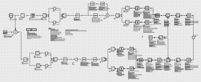 Figure B.1: Schematic of the complete DQPSK/OFDM
system.
Figure B.1: Schematic of the complete DQPSK/OFDM
system.
The schematic shown in Figure B.1 has been
designed with both Numeric and Timed components. Because there does not exist
Timed components for them, the calculation of the Fourier Transform and the
addition/removal of the cyclic prefix have to be implemented in Numeric
components. But as for the GMSK system, it is compulsory to have Timed
components for the up- and down conversion. As we will see later, using both
types of components can lead to some problems of synchronization between the
signals.

Figure B.2:
Schematic of the modulator.
Figure
B.2 shows the modulator part of the system. The bits coming out from the bit
source are mapped into a QPSK constellation on the complex plan. Then they are
differentially encoded. The numeric differential encoder is available only in
the GSM library, which we did not have access to. But we took its scheme, which
we can read, and designed it with ordinary ADS components as it can be seen in
Figure B.3.

Figure B.3: Schematic of the
differential encoder.
The
Inverse Fast Fourier Transform (IFFT) is then applied on the complex data
obtained. The cyclic prefix is added using three CHOP components. The CHOP
permits to divide data into packets. Three major parameters have to be taken
into account: the number of samples read in the input, the number of samples
written in the output and the offset, which is the number of samples the output
is shifted by, compared with the input. If the offset is positive, the samples
are shifted to the right and to the left if it is negative. With this method,
we extract the cyclic prefix from the end of the OFDM symbol and add it at the
beginning of this same OFDM symbol. We then obtain an OFDM symbol of the length
256 (number of points of the IFFT) plus the length of the cyclic prefix
(corresponding to the length of the impulse response of the channel). The data
transmitted through the channel are therefore complex coefficients. That is a
linear amplification is needed.

Figure B.4: Schematic of the time
conversion.
In order to be up-converted, the data have to be converted into time.
Figure B.4 shows this conversion processus: the real and the imaginary part of
the signal are converted separately. Each part is sampled with a time step
correponding to the bit rate that is wanted to be simulated. The signal is then
upsampled by a factor 10. Indeed, the channel having a resolution of
1 nanosecond, the signal would not be precise enough to take all the
channel distorsion into account. A Nyquist square root cosine filtering is
applied in order to filter the rectangular symbols and significantly reduce the
spectral bandwidth required for transmission, with minimal degradation to the
system performance. The real and imaginary part are recombined into a complex
signal thanks to a QAM modulator, which includes also an internal oscillator to
modulate the signal onto a carrier frequency, our Intermediate frequency (IF).
The upconversion, the channel and the downconversion are exactly the
same as for the GMSK system.
The signal has to be converted again into numeric for it to be
demodulated. The numeric conversion is the symetric of the time conversion: QAM
demodulator, Nyquist square root cosine filtering, downsampling by the same
factor as for the upsampling and time-to-real conversion.
Figure B.5 shows the demodulator part.
Figure B.5: Schematic of the
demodulator.
The first component of the demodulator chain is a CHOP. It is very
important for the simulation of the system. Indeed, the conversion between time
and numeric, as well as the up- and downconversion, introduce a delay. In the
numeric part, this delay is represented by a number of zero-valued samples
corresponding to the length of the delay. They have to be removed, otherwise
they are taken into account in the FFT calculation intoducing an error. The
CHOP reads then a number of samples equal to the one that are simulated and
writes this number minus the number of samples of the delay, eliminating them
from the beginning of the sample list. This is a tricky solution, but this is
the only one that works. The problem is that this CHOP component slows a lot
the simulations up to several hours, depending on the number of points being
simulated.
The second CHOP component removes the cyclic prefix. Then a complex
gain permits to get an amplitude of the coefficients in accordance with the
ones at the output of the modulator. The calculation of the FFT is performed
before the data are differentially decoded. The decoder component, as the
encoder, has been designed from the schematic of the component of the GSM
library. It can be seen in figure B.6. Data are then parallel-to-serial
converted in order to be compared with the input bits.

Figure B.6: Schematic of the
differential decoder.
APPENDIX C: MATLAB CHANNEL GENERATION PROGRAM
This
code is used in Matlab to generate a random channel based on the model
described in Chapter 2 section 4.
%------------------------------------------------------------------------------
% Channel generated from the
Saleh model
%------------------------------------------------------------------------------
clear
all
alpha=3; %
Attenuation factor
landa=1/5E-9; % Ray
Arrival rate
gamma_M=20E-9; % Power decay
rate of the first rays
landa_M=1/75E-9; % Cluster
arrival rate
gamma=9E-9; %
Power decay rate within a cluster
r=10; %
Distance
G=power((5E-3/(4*pi)),2);
number_of_cluster=1;
Tl=1/landa_M;
arrival_time=0;
indice_ray=0;
random_variable1=0;
%------------------------------------------------------------------------------
% Average
power of the first ray
%------------------------------------------------------------------------------
Mean_of_Beta_square_00=power(landa*gamma,-1)*G*power(r,-alpha);
%------------------------------------------------------------------------------
% Generation of the rays
arrival times and ray amplitudes (10 rays)
%------------------------------------------------------------------------------
arrival_time_ray=0;
n=(1:10);
factorielle_n=cumprod(1:10);
p_nb_ray=power((1/landa*landa_M),n).*exp(-1/landa*landa_M)./factorielle_n;
for
i=1:number_of_cluster,
random_variable1=rand(1,10);
indice_ray=length(find(p_nb_ray>random_variable1));
if
indice_ray==0
number_of_ray=10;
else
number_of_ray=length(indice_ray(1)+1);
end %
end if
end %
end for
inter_arrival_time_ray=exprnd1(1/landa,1,number_of_ray);
arrival_time_ray(1)=0;
for
i=2:number_of_ray,
arrival_time_ray(i)=arrival_time_ray(i-1)+inter_arrival_time_ray(i-1);
end
Mean_of_Beta_square_kl=Mean_of_Beta_square_00*exp(-arrival_time/gamma_M).*exp(-arrival_time_ray./gamma);
amplitude(2:number_of_ray)=raylrnd1(Mean_of_Beta_square_kl(1:9));
amplitude(1)=Mean_of_Beta_square_00;
j=complex(0,1);
phase=2*pi*rand(1,length(amplitude));
% Generation of the rays phase
retard=round(arrival_time_ray/1E-9);
coefficients=zeros(1,retard(length(retard)));
coefficient_complex=amplitude.*exp(j*phase);
coefficients(1)=amplitude(1);
coefficients(retard+1)=coefficient_complex;
REFERENCES
Wireless
Network and the 60 GHz issue
[1]
Luis M. Correia, Ramjee Prasad, “An Overview of Wireless Broadband
Communications”, IEEE Commun. Mag. January 1997 pp 28-33.
[2]
R. Overduin, P.F.M. Smulders, “Feasibility of Boadband Inroom Radio
Communications at 60 GHz”, Proc. PIMRC 94,
The Hague, The Netherlands, Sept. 1994, pp 119-126.
[3] J.
Fernandes, “Transmission Capacity of a Broadband Wireless Radio Link”, IEEE, RAWCON’98 Proceedings, pp.
149-152, 1998.
[4] M. Chiani,
D. Dardari, A. Zanella and O. Andrisano, “Service Availability of Broadband
Wireless Networks for Indoor Multimedia at Millimetre Waves”, IEEE, 1998.
[5] A. Kato, T.
Manabe, T. Ihara and M. Fujise, “Development and Evaluation on the
Millimeter-wave Indoor Wireless LAN Demonstrators”, IEEE, 1998.
[6] Harry Leib, “A digital transmission approach for indoor
millimetre waveband systems“, IEEE
ICUPC’93, 1993.
[7] M. Pröegler, A. Gusmao, D. Petras, J. Sten, “Deliverable R2067
for the MBS project, Air Interface Final Results”, M. Pröegler, 1995.
[8] Y. Takimoto, T. Ihara, “Research activities on millimetre wave
indoor communication systems in Japan”, IEEE
MTT-S Digest, 1993.
channel modelling
[9] A.A.M.
Saleh and R.A. Valenzuela, “A Statistical Model For Indoor Multipath
Propagation”, IEEE, Journal on selected
areas in communications, vol. SAC-5, No. 2, pp. 128-137, Feb. 1987.
[10] P.F.M.
Smulders and A.G. Wagemans, “A Statistical Model for the mm-wave Indoor Radio
Channel”, IEEE, 1992.
[11] P.F.M. Smulders, L.M. Correia, “Characterisation of Propagation
in 60 GHz radio Channels”, IEEE,
1996.
[12] J.H. Park, Y. Kim, Y.S. Hur, K. Lim and K.H. Kim, “Analysis of
60 GHz Band Indoor Wireless Channels with Channel Configurations”, IEEE, 1998.
[13] S.Y. Seidel, K.Takamizawa, T.H. Rappaport, “Application of
second order statistics for an indoor radio channel model”, IEEE, 1989.
[14] M. Bensebti, J.P. McGeehan, M.A. Beach, “Indoor Multipath Radio
Propagation Measurements and Characterisation at 60 GHz”, ?.
[15] D.S.
Polydorou and C.N. Capsalis, “A New Theoritical Model for the Prediction of
Rapid Fading Variations in a Indoor Environment”, IEEE Transactions on
Vehicular Technology, Vol. 46, No. 3, pp. 748-754, Aug. 1997.
[16] T. Takeuchi, M Sako, S. Yoshida, “Multipath Delay Estimation
for Indoor Wireless Communication”, IEEE,
1990.
[17] Q. Spencer, M. Rice, B. Jeffs, M. Jensen, “A Statistical Model
for Angle of Arrival in Indoor Multipath Propagation”, IEEE, 1997.
[18] L.M. Correia, J.R. Reis, “Wideband Characterisation of the
Propagation Channel for Outdoors at 60 GHz”, IEEE, 1996.
[19] L.M. Correia, J.R. Reis, P.O. Frances, “Analysis of the Average
Power ro Distance Decay Rate at the 60 GHz Band”, IEEE, 1997.
[20] P.
Vasconcelos, L.M. Correia, “Fading Dependence on Scenario and Antennas
Characteristics at the 60 Ghz band”, IEEE
VTC’98, 1998.
[21] J. Hubner,
S. Zeisberg, K Koora, J. Borowski, A. Finger, “Simple Channel Model for 60 GHz
Indoor Wireless LAN design Based on Complex Wideband Measurements”, IEEE, 1997.
modulation and coding performance
[22] J. Sun and I.S.
Reed, “Performance of MDPSK, MPSK and Noncoherent MFSK in Wireless Rician
Fading Channels”, IEEE Transactions on
Communications, Vol. 47, No. 6, pp. 813-816, Jun. 1999.
[23] M. Chiani and A. Volta, “Hybrid ARQ/FEC Techniques for Wireless
ATM Local Area Networks”, IEEE, 1996.
[24] M. Kobayashi, T. Arita, T. Udagawa and M. Nakagawa, “Multi-spot
Diversity Using OFDM for 60 GHz Indoor Wireless LAN”, IEEE ICPWC’99, 1999.
[25] Scott L.Miller, Robert J. O’Dea, “Multiple Symbol Noncoherent
Detection of GMSK”, IEEE, 1998.
[26] Gee L. Lui, “Threshold Detection Performances of GMSK signal
with BT=0.5”, IEEE, 1998.
[27] G.K.Kaleh, “Simple Coherent Receivers for Partial Response
Continuous Phase Modulation”, IEEE,
1989.
[28] M. Kocatürk, S.C. Gupta, H. Arslan,
“Bit-error Rate of TDMA Links under Cochannel Interference in Overlaid Cellular
Networks”, IEEE transactions on vehicular
technology, 1998.
[29] Thomas H. Williams, “A Digital Transmission System with Very
High
Immunity to Dynamic Multipath Distorsion”, IEEE Transactions on broadcasting, pp. 11-19, 1999.
[30] W.A.C Fernando, R.M.A.P. Rajatheva, K.M. Ahmed, “Performance of
Coded OFDM with Higher Modulation Schemes”, IEEE
ICCT’98, 1998.
[31] Robert L. Howald, Stan
Kesler, Moshe Kam, “BER Performance Analysis of OFDM-QAM in Phase Noise”, IEEE , 1998.
[32] C.S. Bontu, David D. Falconer, Leo Strawczynski, “Feasibility
Evaluation of High Rate FSK Data Transmission And Equalization for Millimeter
Wave Indoor Radio”, IEEE, 1996.
[33] F. Gaggioli, Luis M. Correia, “Assessment of Diversity
Performance from Measured data at the Millimetre Waveband”, IEEE VTC’98, pp. 1795-1799, 1998.
[34] B. T. Thoma, T.S. Rappaport, M. D. Keitz, “Simulation of Bit
Error Performance and Outage Probability of p/4 DQPSK in
Frequency-Selective Indoor Radio Channels using a Measurement-Based Channel
Model”, IEEE, 1992.
[35] R.O. Farley, G.M. Stamatelos, D.D. Falconer, “Simulation
Studies of Broadband Wireless Systems Employing Code Combining Techniques”, IEEE, 1996.
[36] P.F.M. Smulders, “Error Control in ATM-Based Indoor Radio
LANS”, IEEE PIMRC’94, 1994.
[37] F. Poegel, S. Zeisberg, A. Finger, “Comparison of Different
Coding Schemes for High Bit Rate OFDM in a 60 GHz environment”, IEEE, 1996.
[38] M. Sandell, S.K. Wilson. P.O. Börjesson, “Performance Analysis of Coded OFDM on Fading
Channels with Non-Ideal Interleaving and Channel Knowledge”, IEEE VTC’97, 1997.
[39] W. Tomaselli, S. Benedetto, “Performance analysis of two
digital wireless systems designed for voice and data transmissions on the
Rayleigh fading channel”, IEEE, 1998.
Multiple Access and Duplexing Methods
[40] H. Harada, R Prasad, “Cyclic Extended Spread Coded Multicarrier
CDMA/TDD Transmission Scheme for Wireless Broadband Multimedia Application”, IEEE VTC’98, pp. 1899-1904, 1998.
[41] M. Jankiraman, R. Prasad, “Hybrid CDMA/OFDM/SFH : A Novel
solution for Wideband Multimedia Communications”,?.
[42] C. Caini, A. Vanelli Coralli, “Coverage Analysis of a DS Spread
Spectrum System over 900 MHz and 60 GHz Indoor Channels”, IEEE, 1998.
[43] A. S. Mahmoud, David D. Falconer, S. A. Mahmoud, “A Multiple
Access Scheme for Wireless Access to a Broadband ATM LAN Based on Polling and
Sectored Antennas”, IEEE, 1995.
[44] C.G. Zhang, H.M. Hafez, D.D. Falconer, “Traffic Handling
Capability of a Broadband Indoor Wireless Network using CDMA Multiple Access”, IEEE journals on selected topics in
communications, 1994.
[45] D. Yu, D.D. Falconer, H.M. Fates, “Traffic Capacity Study of
TDMA In-Building Wireless Systems”, IEEE
ICUPC’93, 1993.
[46] C. Caini, M.L. Merani, A. Vanelli Coralli, “Performance
Evaluation of a DS Spread Spectrum over a 60 GHz Multipath Channel”, IEEE VTC’98, 1998.
[47] J. Brecht, L. Hanzo, “Statistical Packet Assignment Multiple
Access for Wireless Asynchronous Transfer Mode Systems”, IEEE proceedings for ACTS summit’97, 1997.
[48] I. Crohn, G. Schultes, R. Gahleitner, E. Bonek, “Irreducible
Error Performance of a Digital Portable Communication System in a Controlled
Time-Dispersion Indoor Channel”, IEEE
journals on selected areas in communications, 1993.
[49] P.F.M Smulders, “Application of the asynchronous transfer mode
in indoor radio networks”, IEEE/ICCC,
19?.
[50] M.Chiani, D. Dardari, A. Zanella, O. Andrisano, “Service
Availability of Broadband Wireless Networks for Indoor Multimedia at Millimetre
Waves”, IEEE, 1998.
Measurements of propagation parameters at 60 ghz
[51] A.Kato, T.Manabe, Y. Miura, K.Sato, T.Ihara, “Measurements of
Millimeter Wave Indoor Propagation and High Speed Digital Transmission
Characteristics at 60 GHz”, IEEE,
1997.
[52] K.Sato et al,
“Measurements of Reflection and Transmission Characteristics of Interior
Structures of Office Building in the 60-GHz band”, IEEE, 1997.
[53] T. Manabe et al,
“Polarization Dependence of Multipath Propoagation and High-Speed Transmission
Characteristics of Indoor Millimeter-Wave Channel at 60 GHz”, IEEE, 1995.
[54] T. Manabe et al,
“Effects of Antenna Directivity and Polarization on Indoor Multipath
Propagation Characteristics at 60 GHz”, IEEE,
1996.
[55] K.Sato et al,
“Measurement of the Complex Refractive Index of Concrete at 57.5 GHz”, IEEE, 1996.
[56]
S.Haykin, “ Digital Communications”, John
Wiley and Sons, 1988.
[57]
Theodore S. Rappaport, “Wireless Communications, Principles and Practice”, Prentice Hall, 1996.
[58] J.G. Proakis, “Digital Communications”, McGraw Hill, 1995
[59] W. Stallings, “Data and Computer Communications”, Prentice Hall, 1997.
[60] L.W. Couch II, “Digital and Analog Communication Systems”, Mc Millan, 1990.
[61] S. Lin, D.J. Costello, “Error Control Coding : Fundamentals and
Applications”, Prentice Hall, 1983.
[62] P.F.M. Smulders, “Broadband Wireless LAN : a Feasibility
study”, Ph.D. Thesis, Technische
Universiteit Eindhoven, 1995.
[63] D.Bengtsson, D. Landström, “Coding in a Discrete Multitone
Modulation System”, M.Sc. thesis,
1996.
[64] O. Edfors, M, Sandell, Jan Jaap van de Beek, D. Landström, F.
Sjöberg, “An introduction to orthogonal frequency-division multiplexing”.

